Databricks recently announced that it is now also supporting Azure Active Directory Authentication for the REST API which is now in public preview. This may not sound super exciting but is actually a very important feature when it comes to Continuous Integration/Continuous Delivery pipelines in Azure DevOps or any other CI/CD tool. Previously, whenever you wanted to deploy content to a new Databricks workspace, you first needed to manually create a user-bound API access token. As you can imagine, manual steps are also bad for otherwise automated processes like a CI/CD pipeline. With Databricks REST API finally supporting Azure Active Directory Authentication of regular users and service principals, this last manual step is finally also gone!
As I had this issue at many of my customers where we had already fully automated the deployment of our data platform based on Azure and Databricks, I also wanted to use this new feature there. The deployment of regular Databricks objects (clusters, notebooks, jobs, …) was already implemented in the CI/CD pipeline using my PowerShell module DatabricksPS and of course I did not want to rewrite any of those steps. So, I simply extend the module’s authentication methods to also support Azure Active Directory Authentication. The only thing that actually changed was the call to Set-DatabricksEnvironment which now supports additional parameter sets and parameters:
The first thing you will realize is that it is now necessary to specify the Databricks Workspace explicitly either using SubscriptionID/ResourceGroupName/WorkspaceName to uniquely identify the Databricks workspace within Azure or using the OrganizationID that you see displayed in the URL of your Databricks Workspace. For the actual authentication the parameters -ClientID, -TenantID, -Credential and the switch -ServicePrincipal are used.
Regardless of whether you use regular username/password authentication with an AAD user or an AAD service principal, the first thing you need to do in both cases is to create an AAD Application as described in the official docs from Databricks: Using Azure Active Directory Authentication Library Using a service principal
Once you have ensured all prerequisites exist, you can use the samples below to authenticate with your AAD username/password with DatabricksPS:
As you can see, once the environment is set up using the new authentication methods, the rest of the script stays the same and there is not much more you need to do fully automate your CI/CD pipeline with DatabricksPS!
I have not yet fully tested all cmdlets of the module so if you experience any issues, please contact me or open a ticket in the GIT repository.
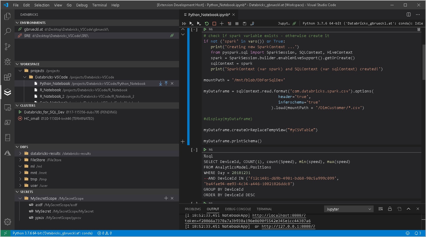
When working with Databricks you will usually start developing your code in the notebook-style UI that comes natively with Databricks. This is perfectly fine for most of the use cases but sometimes it is just not enough. Especially nowadays, where a lot of data engineers and scientists have a strong background also in regular software development and expect the same features that they are used to from their original Integrated Development Environments (IDE) also in Databricks.
For those users Databricks has developed Databricks Connect (Azure docs) which allows you to work with your local IDE of choice (Jupyter, PyCharm, RStudio, IntelliJ, Eclipse or Visual Studio Code) but execute the code on a Databricks cluster. This is awesome and provides a lot of advantages compared to the standard notebook UI. The two most important ones are probably the proper integration into source control / git and the ability to extend your IDE with tools like automatic formatters, linters, custom syntax highlighting, …
While Databricks Connect solves the problem of local execution and debugging, there was still a gap when it came to pushing your local changes back to Databricks to be executed as part of a regular ETL or ML pipeline. So far you had to either “deploy” your changes by manually uploading them via the Databricks UI again or write a script that uploads it via the REST API (Azure docs).
NOTE: I also published a PowerShell module that eases the automation/scripting of these tasks also as part of CI/CD pipeline. It is available from the PowerShell gallery DatabricksPS and integrates very well with this VSCode extension too!
However, this is not really something you would call a “seamless experience” so I also started working on an extension for Visual Studio Code to work more efficiently with Databricks. It has been in the VS Code gallery (Databricks VSCode) for about a month now and I received mostly positive feedback so far. Now I am at a stage where I want to get more people to use it – hence this blog post to announce it officially. The extension is currently published under GPLv3 license and is free to use for everyone. The GIT repository is also linked in the VS Code gallery if you want to participate or have any issues with the extension.
It currently supports the following features:
Workspace browser
Up-/download of notebooks and whole folders
Compare/Diff of local vs online notebook (currently only supported for raw files but not for notebooks)
Execution of local code and notebooks against a Databricks Cluster (via Databricks-Connect)
Cluster manager
Start/stop clusters
Script cluster definition as JSON
Job browser
Start/stop jobs
View job-run history + status
Script job definition as JSON
Script job-run output as JSON
DBFS browser
Upload files
Download files
(also works with mount points!)
Secrets browser
Create/delete secret scopes
Create/delete secrets
Support for multiple Databricks workspaces (e.g. DEV/TEST/PROD)
Easy configuration via standard VS Code settings
More features to come in the future but these will be mainly based on the requests that come from users or my personal needs. So your feedback is highly appreciated – either directly here or using the feedback section in the GIT repository.
I will also write some follow up post to show you how to work in the most efficient way using this new VSCode extension in combination with your Databricks workspace so stay tuned!
One of the most requested features when it comes to Azure ML is and has always been the integration into PowerBI. By now we are still lacking a native connector in PowerBI which would allow us to query a published Azure ML web service directly and score our datasets. Reason enough for me to dig into this issue and create some Power Query M scripts to do this. But lets first start off with the basics of Azure ML Web Services.
Every Azure ML project can be published as a Web Service with just a single click. Once its published, it can be used like any other Web Service. Usually we would send a record or a whole dataset to the Web Service, the Azure ML models does some scoring (or any other operation within Azure ML) and then sends the scored result back to the client. This is straight forward and Microsoft even supplies samples for the most common programming languages. The Web Service relies on a standardized REST API which can basically be called by any client. Yes, in our case this client will be PowerBI using Power Query. Rui Quintino has already written an article on AzureML Web Service Scoring with Excel and Power Query and also Chris Webb wrote a more generic one on POST Request in Power Query in general Web Service and POST requests in Power Query. Even Microsoft recently published an article how you can use the R Integration of Power Query to call a Azure ML Web Service here.
Having tried these solutions, I have to admit that they have some major issues: 1) very static / hard coded 2) complex to write 3) operate on row-by-row basis and might run into the API Call Limits as discussed here. 4) need a local R installation
As Azure ML usually deal with tables, which are basically Power Query DataSets, a requirement would be to directly use a Power Query DataSet. The DataSet has to be converted dynamically into the required JSON structure to be POSTed to Azure ML. The returned result, usually a table again, should be converted back to a Power Query DataSet. And that’s what I did, I wrote a function that does all this for you. All information that you have to supply can be found in the configuration of your Azure ML Web Service: – Request URI of your Web Service – API Key – the [Table to Score]
the [Table to Score] can be any Power Query table but of course has to have the very same structure (including column names and data types) as expected by the Web Service Input. Then you can simply call my function:
The whole process involves a lot of JSON conversions and is kind of complex but as I encapsulated everything into M functions it should be quite easy to use by simply calling the CallAzureMLService-function.
However, here is a little description of the used functions and the actual code:
ToAzureMLJson – converts any object that is passed in as an argument to a JSON element. If you pass in a table, it is converted to a JSON-array. Dates and Numbers are formatted correctly, etc. so the result can the be passed directly to Azure ML.
Default
1
2
3
4
5
6
7
8
9
10
11
12
13
14
15
16
17
18
19
20
21
22
23
24
25
26
27
28
29
30
31
32
33
34
35
36
37
38
39
40
41
42
43
44
45
46
47
48
49
50
51
52
53
54
55
56
let
ToAzureMLJson= (input as any) as text =>
let
transformationList = {
[Type = type time, Transformation = (value_in as time) as text => """" & Time.ToText(value_in, "hh:mm:ss.sss") & """"],
[Type = type date, Transformation = (value_in as date) as text => """" & Date.ToText(value_in, "yyyy-MM-dd") & """"],
[Type = type datetime, Transformation = (value_in as datetime) as text => """" & DateTime.ToText(value_in, "yyyy-MM-ddThh:mm:ss.sss" & """")],
[Type = type datetimezone, Transformation = (value_in as datetimezone) as text => """" & DateTimeZone.ToText(value_in, "yyyy-MM-ddThh:mm:ss.sss") & """"],
[Type = type duration, Transformation = (value_in as duration) as text => ToAzureMLJson(Duration.TotalSeconds(value_in))],
[Type = type number, Transformation = (value_in as number) as text => Number.ToText(value_in, "G", "en-US")],
[Type = type logical, Transformation = (value_in as logical) as text => Logical.ToText(value_in)],
[Type = type text, Transformation = (value_in as text) as text => """" & value_in & """"],
[Type = type record, Transformation = (value_in as record) as text =>
[Type = type list, Transformation = (value_in as list) as text => ToAzureMLJson(Table.FromList(value_in, Splitter.SplitByNothing(), {"ListValue"}, null, ExtraValues.Error))],
[Type = type binary, Transformation = (value_in as binary) as text => """0x" & Binary.ToText(value_in, 1) & """"],
[Type = type any, Transformation = (value_in as any) as text => if value_in = null then "null" else """" & value_in & """"]
},
transformation = List.First(List.Select(transformationList , each Value.Is(input, _[Type]) or _[Type] = type any))[Transformation],
result = transformation(input)
in
result
in
ToAzureMLJson
AzureMLJsonToTable – converts the returned JSON back to a Power Query Table. It obeys column names and also data types as defined in the Azure ML Web Service output. If the output changes (e.g. new columns are added) this will be taken care of dynamically!
Default
1
2
3
4
5
6
7
8
9
10
11
12
13
14
15
16
17
18
19
20
21
22
23
24
25
26
27
28
29
30
31
32
33
34
let
AzureMLJsonToTable = (azureMLResponse as binary) as any =>
CallAzureMLService – uses the two function from above to convert a table to JSON, POST the JSON to Azure ML and convert the result back to a Power Query Table.
Default
1
2
3
4
5
6
7
8
9
10
11
12
13
14
15
16
17
18
19
20
21
22
23
24
let
CallAzureMLService = (
WebServiceURI as text,
WebServiceKey as text,
TableToScore as table,
optional Timeout as number
) as any =>
let
WebTimeout = if Timeout = null then #duration(0,0,0,100) else #duration(0,0,0,Timeout) ,
Known Issues: As the [Table to Score] will probably come from a SQL DB or somewhere else, you may run into issues with Privacy Levels/Settings and the Formula Firewall. In this case make sure to enable Fast Combine for your workbook as described here.
The maximum timeout of a Request/Response call to an Azure ML Web Service is 100 seconds. If your call exceeds this limit, you might get an error message returned.I ran a test and tried to score 60k rows (with 2 numeric columns) at once and it worked just fine, but I would assume that you can run into some Azure ML limits here very easily with bigger data sets. As far as I know, these 100 seconds are for the Azure ML itself only. If it takes several minutes to upload your dataset in the POST request, than this is not part of this 100 seconds. If you are still hitting this issue, you could further try to split your table into different batches, score them separately and combine the results again afterwards.
So these are the steps that you need to do in order to use your Azure ML Web Service together with PowerBI: 1) Create an Azure ML Experiment (or use an existing) 2) Publish the Experiment as a Web Service 3) note the URL and the API Key of your Web Service 4) run PowerBI and load the data that you want to score 5) make sure that the dataset created in 4) has the exact same structure as expected by Azure ML (column names, data types, …) 6) call the function “CallAzureMLWebService” with the parameters from 3) and 5) 7) wait for the Web Service to return the result set 8) load the final table into PowerBI (or do some further transformations before)
And that’s it!
Download: You can find a PowerBI workbook which contains all the functions and code here: CallAzureMLWebService.pbix I used a simple Web Service which takes 2 numeric columns (“Number1” and “Number2”) and returns the [Number1] * [Number2] and [Number1] / [Number2]
PS: you will not be able to run the sample as it is as I changed the API Key and also the URL of my original Azure ML Web Service
One of the coolest features of Power BI is that I integrates very well with other tools and also offers a lot of interfaces which can be used to extend this capabilities even further. One of those is the R Integration which allows you to run R code from within Power BI. R scripts can either be used as a data source or for visualizing your data. In this post I will focus on the data source component and show how you can use a locally stored R script and execute it directly in Power BI. Compared to the native approach where you need to embed the R code in the Power BI file, this has several advantages:
Develop R script in familiar external tool like RStudio
Integration with Source Control
Leverage Power BI for publishing and visualizing results
Out of the box Power BI only supplies one function to call R scripts as a data source which is R.Execute(text). Usually, when you use the wizard, it simply passes your R script as a hardcoded value to this function. Knowing the power of Power BI and its scripting language M for data integration made me think – “Hey, as R scripts are just text files and Power BI can read text files, I could also dynamically read any R script and execute it!”
Well, turns out to be true! So I created a little M function where I pass in the file-path of an existing R script and which returns a table of data frames which are created during the execution of the script. Those can then be used like any other data sets/tables within Power BI:
And here is the corresponding M code for the Power Query function: (Thanks also to Imke Feldmann for simplifying my original code to the readable one below)
let
LoadLocalRScript = (file_path as text) as table =>
First we read the R script like any other regular CSV file but we use line-feed (“#(lf)”) as delimiter. So we get a table with one column and one row for each line of our original R script. Then we use Text.Combine() on our column to transform the single lines back into one long text resembling our original R script. This text can the be passed to the R.Execute() function to return the list of R data frames created during the execution of the script.
And that’s it! Any further steps are similar to using any regular R script which is embedded in Power BI so it is up to you on how you proceed from here. Just one thing you need to keep in mind is that changing the local R script might break the Power BI load if you changed or deleted any data frames which are referenced in Power BI later on.
One issues that I came across during my tests is that this approach does not work with scheduled refreshes in the Power BI Web Service via the Personal Gateway. The first reason for this is that it is currently not possible to use scheduled refresh if custom functions are involved. Even if you can work around this issue pretty easily by using the code from above directly in Power Query I still ran into issues with different privacy levels for the location of the R script and the R.Execute() function. But I will investigate into those issues and update this blog post accordingly (see UPDATE below). For the future I hope that is fixed by Microsoft and Power BI allows you to execute remote scripts natively – but until then, this approach worked quite well for me.
UPDATE: To make the refresh via the Personal Gateway work you have to enable “FastCombine”. How to do this is described in more detail here: Turn on FastCombine for Personal Gateway.
In case you are interested in more details on this approach, I am speaking at TugaIT in Lisbon, Portugal this Friday (20th of May 2016) about “Power BI for the Data Scientist” where I will cover this and lots of other interesting topics about the daily work of a data scientist and how PowerBI can used to ease them.
The original request for this calculation came from one of my blog readers who dropped me a mail asking if it possible to calculated the Pearson Correlation Coefficient (PCC or PPMCC) in his PowerPivot model. In case you wonder what the Pearson Correlation Coefficient is and how it can be calculated – as I did in the beginning – these links What is PCC, How to calculate PCC are very helpful and also offer some examples and videos explaining everything you need to know about it. I highly recommend to read the articles before you proceed here as I will not go into the mathematical details of the calculation again in this blog which is dedicated to the DAX implementation of the PCC.
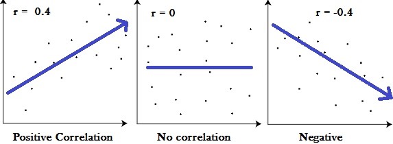
Anyway, as I know your time is precious, I will try to sum up its purpose for you: “The Pearson Correlation Coefficient calculates the correlation between two variables over a given set of items. The result is a number between -1 and 1. A value higher than 0.5 (or lower than –0.5) indicate a strong relationship whereas numbers towards 0 imply weak to no relationship.”
The two values we want to correlate are our axes, whereas the single dots represent our set of items. The PCC calculates the trend within this chart represented as an arrow above.
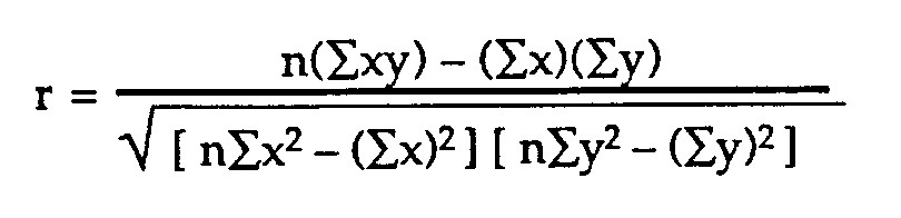
The mathematical formula that defines the Pearson Correlation Coefficient is the following:
The PCC can be used to calculate the correlation between two measures which can be associated with the same customer. A measure can be anything here, the age of a customer, it’s sales, the number of visits, etc. but also things like sales with red products vs. sales with blue products. As you can imagine, this can be a very powerful statistical KPI for any analytical data model. To demonstrate the calculation we will try to correlate the order quantity of a customer with it’s sales amount. The order quantity will be our [MeasureX] and the sales will be our [MeasureY], and the set that we will calculate the PCC over are our customers. To make the whole calculation more I split it up into separate measures:
MeasureX := SUM(‘Internet Sales’[Order Quantity])
MeasureY := SUM(‘Internet Sales’[Sales Amount])
Based on these measures we can define further measures which are necessary for the calculation of our PCC. The calculations are tied to a set if items, in our case the single customers:
Now that we have calculated the various summations over our base measures, it is time to create the numerator and denominator for our final calculation:
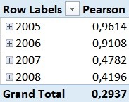
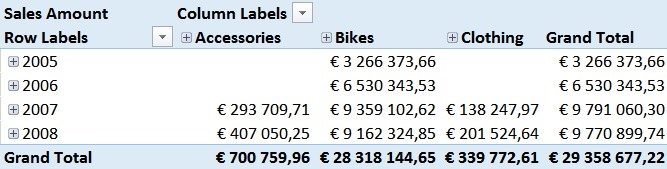
This [Pearson]-measure can then be used together with any attribute in our model – e.g. the Calendar Year in order to track the changes of the Pearson Correlation Coefficient over years:
Pearson by Year
For those of you who are familiar with the Adventure Works sample DB, this numbers should not be surprising. In 2005 and 2006 the Adventure Works company only sold bikes and usually a customer only buys one bike – so we have a pretty strong correlation here. However, in 2007 they also started selling Clothing and Accessories which are in general cheaper than Bikes but are sold more often.
Pearson by Year and Category
This has impact on our Pearson-value which is very obvious in the screenshots above.
As you probably also realized, the Grand Total of our Pearson calculation cannot be directly related to the single years and may also be the complete opposite of the single values. This effect is called Simpson’s Paradox and is the expected behavior here.
[MeasuresX] and [MeasureY] can be exchanged by any other DAX measures which makes this calculation really powerful. Also, the set of items over which we want to calculated the correlation can be exchanged quite easily. Below you can download the sample Excel workbook but also a DAX query which could be used in Reporting Services or any other tool that allows execution of DAX queries.