The original request for this calculation came from one of my blog readers who dropped me a mail asking if it possible to calculated the Pearson Correlation Coefficient (PCC or PPMCC) in his PowerPivot model. In case you wonder what the Pearson Correlation Coefficient is and how it can be calculated – as I did in the beginning – these links What is PCC, How to calculate PCC are very helpful and also offer some examples and videos explaining everything you need to know about it. I highly recommend to read the articles before you proceed here as I will not go into the mathematical details of the calculation again in this blog which is dedicated to the DAX implementation of the PCC.
UPDATE 2017-06-04:
Daniil Maslyuk posted an updated version of the final calculation using DAX 2.0 which is much more readable as it is using variables instead of separate measures for every intermediate step. His blog post can be found at https://xxlbi.com/blog/pearson-correlation-coefficient-in-dax/
Anyway, as I know your time is precious, I will try to sum up its purpose for you: “The Pearson Correlation Coefficient calculates the correlation between two variables over a given set of items. The result is a number between -1 and 1. A value higher than 0.5 (or lower than –0.5) indicate a strong relationship whereas numbers towards 0 imply weak to no relationship.”
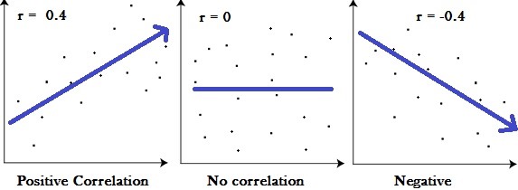
The two values we want to correlate are our axes, whereas the single dots represent our set of items. The PCC calculates the trend within this chart represented as an arrow above.
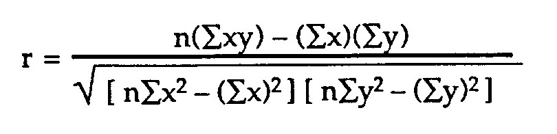
The mathematical formula that defines the Pearson Correlation Coefficient is the following:
The PCC can be used to calculate the correlation between two measures which can be associated with the same customer. A measure can be anything here, the age of a customer, it’s sales, the number of visits, etc. but also things like sales with red products vs. sales with blue products. As you can imagine, this can be a very powerful statistical KPI for any analytical data model. To demonstrate the calculation we will try to correlate the order quantity of a customer with it’s sales amount. The order quantity will be our [MeasureX] and the sales will be our [MeasureY], and the set that we will calculate the PCC over are our customers. To make the whole calculation more I split it up into separate measures:
- MeasureX := SUM(‘Internet Sales’[Order Quantity])
- MeasureY := SUM(‘Internet Sales’[Sales Amount])
Based on these measures we can define further measures which are necessary for the calculation of our PCC. The calculations are tied to a set if items, in our case the single customers:
- Sum_XY := SUMX(VALUES(Customer[Customer Id]), [MeasureX] * [MeasureY])
- Sum_X2 := SUMX(VALUES(Customer[Customer Id]), [MeasureX] * [MeasureX])
- Sum_Y2 := SUMX(VALUES(Customer[Customer Id]), [MeasureY] * [MeasureY])
- Count_Items := DISTINCTCOUNT(Customer[Customer Id])
Now that we have calculated the various summations over our base measures, it is time to create the numerator and denominator for our final calculation:
- Pearson_Numerator :=
- ([Count_Items] * [Sum_XY]) – ([MeasureX] * [MeasureY])
- Pearson_Denominator_X :=
- ([Count_Items] * [Sum_X2]) – ([MeasureX] * [MeasureX])
- Pearson_Denominator_Y :=
- ([Count_Items] * [Sum_Y2]) – ([MeasureY] * [MeasureY])
- Pearson_Denominator :=
- SQRT([Pearson_Denominator_X] * [Pearson_Denominator_Y])
Having these helper-measures in place the final calculation for our PCC is straight forward:
- Pearson := DIVIDE([Pearson_Numerator], [Pearson_Denominator])
This [Pearson]-measure can then be used together with any attribute in our model – e.g. the Calendar Year in order to track the changes of the Pearson Correlation Coefficient over years:
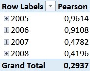
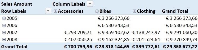
For those of you who are familiar with the Adventure Works sample DB, this numbers should not be surprising. In 2005 and 2006 the Adventure Works company only sold bikes and usually a customer only buys one bike – so we have a pretty strong correlation here. However, in 2007 they also started selling Clothing and Accessories which are in general cheaper than Bikes but are sold more often.
This has impact on our Pearson-value which is very obvious in the screenshots above.
As you probably also realized, the Grand Total of our Pearson calculation cannot be directly related to the single years and may also be the complete opposite of the single values. This effect is called Simpson’s Paradox and is the expected behavior here.
[MeasuresX] and [MeasureY] can be exchanged by any other DAX measures which makes this calculation really powerful. Also, the set of items over which we want to calculated the correlation can be exchanged quite easily. Below you can download the sample Excel workbook but also a DAX query which could be used in Reporting Services or any other tool that allows execution of DAX queries.
Sample Workbook (Excel 2013): Pearson.xlsx
DAX Query: Pearson_SSRS.dax