PowerBI & Big Data – Using pre-calculated Aggregations of Semi- and Non-Additive Measures

Calculating and visualizing semi- and non-additive measures like distinct count in Power BI is usually not a big deal. However, things can become challenging if your data volume grows and exceeds the limits of Power BI!

In one of my recent projects we wanted to visualize data from the customers analytical platform based on Azure Databricks in Power BI. The connection between those two tools works pretty flawless which I also described in my previous post but the challenge was the use-case and the calculations. We wanted to display the distinct customers across various aggregations levels over a billion rows fact table. We came up with different potential solutions all having their pros and cons:

  1. load all data into Power BI (import mode) and do the aggregations there
  2. use Power BI with direct query and let the back-end do the heavy lifting
  3. load only necessary pre-aggregated data into Power BI (import mode)

Please keep in mind that we are dealing with a distinct count measure here. Semi- and Non-additive measure like this cannot easily be aggregated from lower levels to higher levels without having all the detail data available!

Option 1. has the obvious drawback that data model would be huge in size as we were dealing with billions of transactions. This would have exceeded our current size limits for Power BI data models.

Option 2. would usually work fine, but again, for the amount of data we were dealing with the back-end was just no able to provide sub-second latency that was required.

So we went for Option 3. and did the various aggregations on the different levels in Azure Databricks and loaded only the final results to Power BI. First we wanted to use Power BI Aggregations and Composite Models. Unfortunately, this did not work out for us as we were not in control which aggregation table (we had multiple for the different aggregation levels) was used by the engine which potentially resulted in wrong results when additional aggregation was done in Power BI. Also, when slicing for random aggregation levels, Power BI was querying the details in direct query mode causing very poor query performance.

After some further thinking we came up with a new solution which was also based on pre-calculated aggregations but not realized using built-in aggregation tables but having a combined table for all aggregations and some very straight-forward DAX to select the row we wanted! In the end the whole solution consisted of one SQL view using COUNT(DISTINCT xxx) aggregation and GROUP BY GROUPING SETS (T-SQL, Databricks, … supported in all major SQL engines) and a very simple DAX measure!

Here is a little example that illustrates the approach. Assume you want to calculate the distinct customers that bought certain products in a subcategory/category by year. The first step is to create a view that provides this information:

Please note that when we have a natural relationship between hierarchy levels (= only 1:n relationships) we need to specify the current level and also all upper levels to allow a proper drill-down later on! E.g. ProductCategory (1 -> n) ProductSubcategory

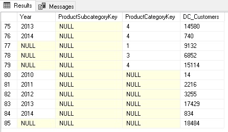
This calculates all the different aggregation levels we need. Columns with NULL mean they were not filtered/grouped by when calculating the aggregation.
Rows 80-84 contain the aggregations grouped by Year only whereas rows 77-79 contain only aggregates by ProductCategoryKey. The rows 75-76 were aggregated by Year AND ProductCategoryKey.
Depending on your final report layout, you may not need all of them and you should consider removing those that are not needed!

This table is then loaded into Power BI. You can either use a custom SQL query like above in Power BI directly or create a view in the back-end system which would be my preferred solution. Alternatively you can also create all these grouping sets using Power Query/M. The incredible Imke Feldmann (t, b) came up with a solution that allows you to specify the grouping sets in a similar way as in SQL and do all this magic within Power BI directly! I hope she will blog about it pretty soon!
(The sample workbook at the end of this post also contains a little preview of this M-magic.)

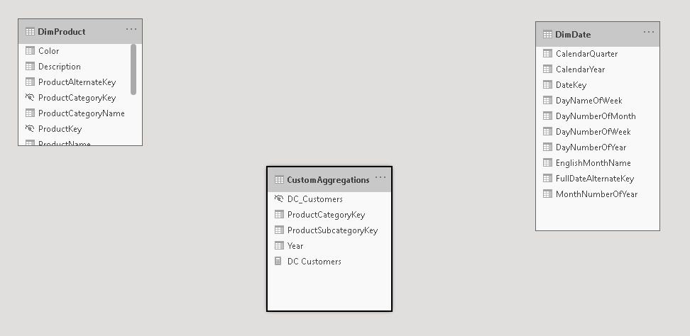
Now that we have all the data we need in Power BI, we need to display the right values for the selections in the report which of course can be dynamic. That’s a bit tricky but once you understand the concept, it is pretty straight forward. First of all, the table containing the aggregations must not be related to any other table as we build them on the fly within our DAX measure. The table itself can also be hidden.

And this is the final DAX for our measure:

The first part is to get all the selected values of the lookup/dimension tables the user selects on the report. These are all the _sel_XXX variables. SELECTEDVALUE() returns the selected value if only one item is in the current filter context and BLANK()/NULL otherwise. We then use TREATAS() to apply those filters (either a single item or NULL) to our aggregations table. This should usually only return a table with a single row so we can use MAXX() to get our actual value from that one row. I also added a check in case multiple rows are returned which can potentially happen if you use multi-selects in your filters and instead of showing wrong values I’d rather indicate that there is something wrong with the calculation.

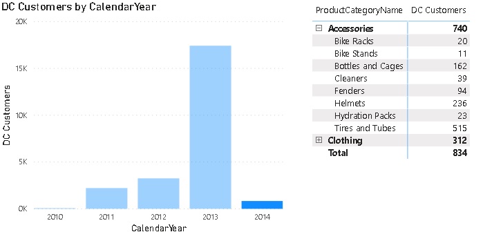
The measure can then be sliced and diced by our pre-defined aggregation levels as if it would be a regular measure but instead of having to process those expensive calculations on the fly we use the pre-calculated aggregates!

One thing to be aware of is that it will produce wrong results if multiple items for any of the aggregation levels are selected so it is highly recommended to set all slicers/filters to single select only or ensure that the filtered aggregation levels are also used in the chart. In this case only the grand total will show wrong values or NULL then.
This could also be fixed in the DAX measure by checking how many rows are actually selected for each level and throw an error in case it is used in a filter and the count of values is > 1.

I did some further thinking and this approach could probably also be used to mimic custom roll-ups and unary operators we know from Analysis Services Multidimensional cubes. If I find some proper examples and this turns out to be feasibly I will write another blog post about it!

Download: Custom_Aggregations_NonAdditive_Measure.pbix

Optimizing Columnar Storage for Measures

First of all I have to thank Marco Russo for his blog post on Optimizing High Cardinality Columns in Vertipaq and also his great session at SQL PASS Rally Nordic in Stockholm last year which taught me a lot about columnar storage in general. I highly recommend everyone to read the two mentioned resources before continuing here. Most of the ideas presented in this post are based on these concepts and require at least basic knowledge in columnar storage.

When writing one of my recent posts I ended up with a Power Pivot model with roughly 40M rows. It contained internet logs from Wikipedia, how often someone clicked on a given page per month and how many bytes got downloaded. As you can imagine those values can vary very heavily, especially the amount of bytes downloaded. So in the Power Pivot model we end up having a lot of distinct values in our column that we use for our measure. As you know from Marcos posts, the allocated memory and therefore also the  performance of columnar storage systems is directly related to the number of distinct values in a column – the more the worse. Marco already described an approach to split up a single column with a lot of distinct values into several columns with less distinct values to optimize storage. These concepts can also be used on columns that contain measures or numeric values in general. Splitting numeric values is quite easy, assuming your values range from 1 to 1,000,000 you can split this column into two by dividing the value by 1000 and using MOD 1000 for the second column. Instead of one column with the value 123,456 you end up with two columns with the values 123 and 456. In terms of storage this means that instead of 1,000,000 distinct values we only need to store 2 x 1,000 distinct values. Nothing new so far.

The trick is to combine those columns again at query time to get the original results as before the split. For some aggregations like SUM this is pretty straight forward, others are a bit more tricky. Though, in general the formulas are not really very complex and can be adopted very easily to handle any number of columns:

Aggregation DAX Formula
Value_SUM1 =SUMX(‘1M_Rows_splitted’, [Value_1000] * 1000 + [Value_1])
Value_SUM2 =SUM ( ‘1M_Rows_splitted'[Value_1000] ) * 1000
    + SUM ( ‘1M_Rows_splitted'[Value_1] )
Value_MAX =MAXX(‘1M_Rows_splitted’, [Value_1000] * 1000 + [Value_1])
Value_MIN =MINX(‘1M_Rows_splitted’, [Value_1000] * 1000 + [Value_1])
Value_COUNT =COUNTX(‘1M_Rows_splitted’, [Value_1000] * 1000 + [Value_1])
Value_DISTINCTCOUNT =COUNTROWS (
    SUMMARIZE (
        ‘1M_Rows_splitted’,
        ‘1M_Rows_splitted'[Value_1000],
        ‘1M_Rows_splitted'[Value_1]))

As you can see you can still mimic most kind of aggregation even if the [Value]-column is split up.

Though, don’t exaggerate splitting your columns – too many may be a bit inconvenient to handle and may neglect the effect resulting in worse performance. Marco already showed that you can get a reduction of up to 90% in size, during my simple tests I came up with about the same numbers. Though, it very much depends on the number of distinct values that you actually have in your column!

I would not recommend to always use this approach for all your measure column – no, definitely not! First check how many distinct values your data/measures contain and decide afterwards. For 1 million distinct values it is probably worth it, for 10,000 you may reconsider using this approach. Most important here is to test this pattern with your own data, data model and queries! Test it in terms of size and of course also in terms of performance. It may be faster to split up columns but it may also be slower and it may be also different for each query that you execute against the tabular model / Power Pivot. Again, test with your own data, data model and queries to get representative results! 

Here is a little test that you may run on your own to test this behavior. Simple create the following Power Query using M, load the result into Power Pivot and save the workbook. It basically creates a table with 1 million distinct values (0 to 999,999) and splits this column up into two. You can just copy the workbook, remove the last step “Remove Columns” and save it again to get the “original” workbook and Power Pivot model.

let
    List1 = List.Numbers(0, 1000000),

    TableFromList = Table.FromList(List1, Splitter.SplitByNothing(), null, null, ExtraValues.Error),
    RenamedColumns = Table.RenameColumns(TableFromList,{{"Column1", "Value"}}),
    ChangedType1 = Table.TransformColumnTypes(RenamedColumns,{{"Value", type number}}),
    InsertedCustom = Table.AddColumn(ChangedType1, "Value_1000", each Number.RoundDown([Value] / 1000)),
    InsertedCustom1 = Table.AddColumn(InsertedCustom, "Value_1", each Number.Mod([Value], 1000)),
    ChangedType = Table.TransformColumnTypes(InsertedCustom1,{{"Value_1000", type number}, {"Value_1", type number}}),
    RemovedColumns = Table.RemoveColumns(ChangedType,{"Value"})
in
    RemovedColumns

This is what I ended up with when you compare those two workbooks:

  # distinct values Final Size
single column 1,000,000 14.4 MB
two columns 2 x 1,000 1.4 MB

We also get a reduction in size of 90%! Though, this is a special scenario …
In the real world, taking my previous scenario with the Wikipedia data as an example, I ended up with a reduction to 50%, still very good though. But as you can see the reduction factor varies very much.

Downloads:

Sample workbook with Power Query: 1M_Rows_splitted.xlsx

Using Power Query to analyze SSAS Disk Usage

Some time ago Bob Duffy blogged about on how to use Power Pivot to analyze the disk usage of multidimensional Analysis Services models (here). He uses a an VBA macro to pull meta data like filename, path, extension, etc. from the file system or to be more specific from the data directory of Analysis Services. Analysis Services stores all its data in different files with specific extensions so it is possible to link those files to multidimensional objects in terms of attributes, facts, aggregations, etc. Based on this data we can analyze  how our data is distributed. Do we have too big dimensions? Which attribute uses the most space? Do our facts consume most of the space (very likely)? If yes, how much of it is real data and how big are my aggregations – if they are processed at all?!? – These are very common and also important things to know for an Analysis Services developer.

So Bob Duffy’s solution can be really useful. The only thing I did not like about it was the fact that it uses a VBA macro to get the data. This made me think and I came up with the idea of using Power Query to get this data. Btw, make sure to check out the latest release, there have been a lot of improvements recently!

With Power Query you have to option to load multiple files from a folder and also from its sub folders. When we do this on our Analysis Services data directory, we get a list of ALL files together with their full path, filename, extension and most important in this case their size which can be found by expanding the Attributes-record:
PQ_Source_FileList

The final Power Query does also a lot of other things to prepare the data so it can be later joined to our FileExtensions-table that holds detailed information for each file extension. This table currently looks like below but can be extended by any other columns that may be necessary and/or useful for you:

FileType FileType_Description ObjectType ObjectTypeSort ObjectTypeDetails
ahstore Attribute Hash Store Dimensions 20 Attribute
asstore Attribute String Store Dimensions 20 Attribute
astore Attribute Store Dimensions 20 Attribute
bsstore BLOB String Store Dimensions 20 BLOB
bstore BLOB Store Dimensions 20 BLOB
dstore Hierarchy Decoding Store Dimensions 20 Hierarchy
khstore Key Hash Store Dimensions 20 Key
ksstore Key String Store Dimensions 20 Key
kstore Key Store Dimensions 20 Key
lstore Structure Store Dimensions 20 Others
ostore Order Store Dimensions 20 Others
sstore Set Store Dimensions 20 Others
ustore ustore Dimensions 20 Others
xml XML Configuration 999 Configuration
fact.data Basedata Facts 10 Basedata
fact.data.hdr Basedata Header Facts 10 Basedata
fact.map Basedata Index Facts 10 Basedata
fact.map.hdr Basedata Index Header Facts 10 Basedata
rigid.data Rigid Aggregation Data Facts 10 Aggregations
rigid.data.hdr Rigid Aggregation Data Header Facts 10 Aggregations
rigid.map Rigid Aggregation Index Facts 10 Aggregations
rigid.map.hdr Rigid Aggregation Index Header Facts 10 Aggregations
flex.data Flexible Aggregation Data Facts 10 Aggregations
flex.data.hdr Flexible Aggregation Data Header Facts 10 Aggregations
flex.map Flexible Aggregation Index Facts 10 Aggregations
flex.map.hdr Flexible Aggregation Index Header Facts 10 Aggregations
string.data String Data (Distinct Count?) Facts 10 Basedata
cnt.bin Binary Configuration 999 Binaries
mrg.ccmap mrg.ccmap DataMining 999 DataMining
mrg.ccstat mrg.ccstat DataMining 999 DataMining
nb.ccmap nb.ccmap DataMining 999 DataMining
nb.ccstat nb.ccstat DataMining 999 DataMining
dt dt DataMining 999 DataMining
dtavl dtavl DataMining 999 DataMining
dtstr dtstr DataMining 999 DataMining
dmdimhstore dmdimhstore DataMining 999 DataMining
dmdimstore dmdimstore DataMining 999 DataMining
bin Binary Configuration 999 Binaries
OTHERS Others Others 99999 Others

As you can see the extension may contain 1, 2 or 3 parts. The more parts the more specific this file extension is. If you checked the result of the Power Query it also contains 3 columns, FileExtension1, FileExtension2 and FileExtension3. To join the two tables we first need to load both tables into Power Pivot. The next step is to create a proper column on which we can base our relationship. If the 3-part extension is found in the file extensions table, we use it, otherwise we check the 2-part extension and afterwards the 1-part extension and in case nothing matches we use “OTHERS”:

=SWITCH(TRUE(),
CONTAINS(FileTypes, FileTypes[FileType], [FileExtension3]), [FileExtension3],
CONTAINS(FileTypes, FileTypes[FileType], [FileExtension2]), [FileExtension2],
CONTAINS(FileTypes, FileTypes[FileType], [FileExtension1]), [FileExtension1],
"OTHERS")

Then we can create a relationship between or PQ table and our file extension table. I also created some other calculated columns, hierarchies and measures for usability. And this is the final outcome:
PivotTable_Report

You can very easily see, how big your facts are, the distribution between base-data and Aggregations, the Dimensions sizes and you can drill down to each individual file! You can of course also create a Power View report if you want to. All visualizations are up to you, this is just a very simple example of a report.

Enjoy playing around with it!

Downloads:
(please note that I added a filter on the Database name as a last step of the Power Query to only show Adventure Works databases! In order to get all databases you need to remove this filter!)

SSAS Disk Analysis Workbook: SSAS_DiskAnalysis.xlsx