Score whole PowerBI DataSets dynamically in Azure ML

One of the most requested features when it comes to Azure ML is and has always been the integration into PowerBI. By now we are still lacking a native connector in PowerBI which would allow us to query a published Azure ML web service directly and score our datasets. Reason enough for me to dig into this issue and create some Power Query M scripts to do this. But lets first start off with the basics of Azure ML Web Services.

Every Azure ML project can be published as a Web Service with just a single click. Once its published, it can be used like any other Web Service. Usually we would send a record or a whole dataset to the Web Service, the Azure ML models does some scoring (or any other operation within Azure ML) and then sends the scored result back to the client. This is straight forward and Microsoft even supplies samples for the most common programming languages. The Web Service relies on a standardized REST API which can basically be called by any client. Yes, in our case this client will be PowerBI using Power Query.
Rui Quintino has already written an article on AzureML Web Service Scoring with Excel and Power Query and also Chris Webb wrote a more generic one on POST Request in Power Query in general Web Service and POST requests in Power Query. Even Microsoft recently published an article how you can use the R Integration of Power Query to call a Azure ML Web Service here.

Having tried these solutions, I have to admit that they have some major issues:
1) very static / hard coded
2) complex to write
3) operate on row-by-row basis and might run into the API Call Limits as discussed here.
4) need a local R installation

As Azure ML usually deal with tables, which are basically Power Query DataSets, a requirement would be to directly use a Power Query DataSet. The DataSet has to be converted dynamically into the required JSON structure to be POSTed to Azure ML. The returned result, usually a table again, should be converted back to a Power Query DataSet. And that’s what I did, I wrote a function that does all this for you. All information that you have to supply can be found in the configuration of your Azure ML Web Service:
– Request URI of your Web Service
– API Key
– the [Table to Score]

the [Table to Score] can be any Power Query table but of course has to have the very same structure (including column names and data types) as expected by the Web Service Input. Then you can simply call my function:
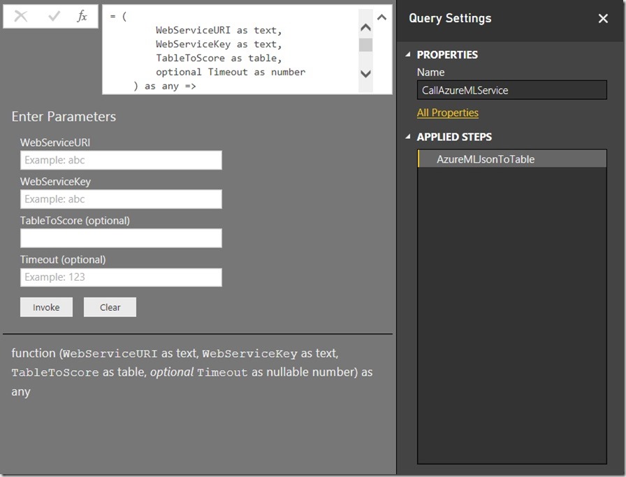
InvokeFunction_PowerBI_DataSet_in_AzureML
Score_PowerBI_DataSet_in_AzureML

The whole process involves a lot of JSON conversions and is kind of complex but as I encapsulated everything into M functions it should be quite easy to use by simply calling the CallAzureMLService-function.

However, here is a little description of the used functions and the actual code:


ToAzureMLJson – converts any object that is passed in as an argument to a JSON element. If you pass in a table, it is converted to a JSON-array. Dates and Numbers are formatted correctly, etc. so the result can the be passed directly to Azure ML.

let
    ToAzureMLJson= (input as any) as text => 
let
    transformationList = {
        [Type = type time, Transformation = (value_in as time) as text => """" & Time.ToText(value_in, "hh:mm:ss.sss") & """"], 
        [Type = type date, Transformation = (value_in as date) as text => """" & Date.ToText(value_in, "yyyy-MM-dd") & """"], 
        [Type = type datetime, Transformation = (value_in as datetime) as text => """" & DateTime.ToText(value_in, "yyyy-MM-ddThh:mm:ss.sss" & """")], 
        [Type = type datetimezone, Transformation = (value_in as datetimezone) as text => """" & DateTimeZone.ToText(value_in, "yyyy-MM-ddThh:mm:ss.sss") & """"], 
        [Type = type duration, Transformation = (value_in as duration) as text => ToAzureMLJson(Duration.TotalSeconds(value_in))], 

        [Type = type number, Transformation = (value_in as number) as text => Number.ToText(value_in, "G", "en-US")],
        [Type = type logical, Transformation = (value_in as logical) as text => Logical.ToText(value_in)],

        [Type = type text, Transformation = (value_in as text) as text => """" & value_in & """"],

        [Type = type record, Transformation = (value_in as record) as text => 
                            let
                                GetFields = Record.FieldNames(value_in),
                                FieldsAsTable = Table.FromList(GetFields, Splitter.SplitByNothing(), {"FieldName"}, null, ExtraValues.Error),
                                AddFieldValue = Table.AddColumn(FieldsAsTable, "FieldValue", each Record.Field(value_in, [FieldName])),
                                AddJson = Table.AddColumn(AddFieldValue, "__JSON", each ToAzureMLJson([FieldValue])),

                                jsonOutput = "[" & Text.Combine(AddJson[__JSON], ",") & "]"
                            in
                                jsonOutput
                            ],
        [Type = type table, Transformation = (value_in as table) as text => 
                            let
                                BufferedInput = Table.Buffer(value_in),
                                GetColumnNames = Table.ColumnNames(BufferedInput),
                                ColumnNamesAsTable = Table.FromList(GetColumnNames , Splitter.SplitByNothing(), {"FieldName"}, null, ExtraValues.Error),
                                ColumnNamesJson = """ColumnNames"": [""" & Text.Combine(ColumnNamesAsTable[FieldName], """, """) & """]",

                                AddJson = Table.AddColumn(value_in, "__JSON", each ToAzureMLJson(_)),
                                ValuesJson = """Values"": [" & Text.Combine(AddJson[__JSON], ",#(lf)") & "]",

                                jsonOutput = "{""Inputs"": { ""input1"": {" & ColumnNamesJson & "," & ValuesJson & "} }, ""GlobalParameters"": {} }"
                            in
                                jsonOutput
                            ],
        [Type = type list, Transformation = (value_in as list) as text => ToAzureMLJson(Table.FromList(value_in, Splitter.SplitByNothing(), {"ListValue"}, null, ExtraValues.Error))],

        [Type = type binary, Transformation = (value_in as binary) as text => """0x" & Binary.ToText(value_in, 1) & """"],


        [Type = type any, Transformation = (value_in as any) as text => if value_in = null then "null" else """" & value_in & """"]

    },

    transformation = List.First(List.Select(transformationList , each Value.Is(input, _[Type]) or _[Type] = type any))[Transformation],

    result = transformation(input)  
in
    result 
in
    ToAzureMLJson

AzureMLJsonToTable – converts the returned JSON back to a Power Query Table. It obeys column names and also data types as defined in the Azure ML Web Service output. If the output changes (e.g. new columns are added) this will be taken care of dynamically!

let
    AzureMLJsonToTable = (azureMLResponse as binary) as any => 
let
    WebResponseJson = Json.Document(azureMLResponse ,1252),
    Results = WebResponseJson[Results],
    output1 = Results[output1],
    value = output1[value],
    BufferedValues = Table.Buffer(Table.FromRows(value[Values])),
    ColumnNameTable = Table.AddIndexColumn(Table.FromList(value[ColumnNames], Splitter.SplitByNothing(), {"NewColumnName"}, null, ExtraValues.Error), "Index", 0, 1),
    ColumnNameTable_Values = Table.AddIndexColumn(Table.FromList(Table.ColumnNames(BufferedValues), null, {"ColumnName"}), "Index", 0, 1),

    RenameList = Table.ToRows(Table.RemoveColumns(Table.Join(ColumnNameTable_Values, "Index", ColumnNameTable, "Index"),{"Index"})),
    RenamedValues = Table.RenameColumns(BufferedValues, RenameList),

    ColumnTypeTextTable = Table.AddIndexColumn(Table.FromList(value[ColumnTypes], Splitter.SplitByNothing(), {"NewColumnType_Text"}, null, ExtraValues.Error), "Index", 0, 1),
    ColumnTypeText2Table = Table.AddColumn(ColumnTypeTextTable, "NewColumnType", each 
     if Text.Contains([NewColumnType_Text], "Int") then type number 
else if Text.Contains([NewColumnType_Text], "DateTime") then type datetime 
else if [NewColumnType_Text] = "String" then type text 
else if [NewColumnType_Text] = "Boolean" then type logical
else if [NewColumnType_Text] = "Double" or [NewColumnType_Text] = "Single" then type number
else if [NewColumnType_Text] = "datetime" then type datetime
else if [NewColumnType_Text] = "DateTimeOffset" then type datetimezone
else type any),
    ColumnTypeTable  = Table.RemoveColumns(ColumnTypeText2Table ,{"NewColumnType_Text"}),  
    
    DatatypeList = Table.ToRows(Table.RemoveColumns(Table.Join(ColumnNameTable, "Index", ColumnTypeTable, "Index"),{"Index"})),
    RetypedValues = Table.TransformColumnTypes(RenamedValues, DatatypeList, "en-US"),
    
    output = RetypedValues
in
    output 
in
    AzureMLJsonToTable

CallAzureMLService – uses the two function from above to convert a table to JSON, POST the JSON to Azure ML and convert the result back to a Power Query Table.

let
    CallAzureMLService = (
        WebServiceURI as text,
        WebServiceKey as text,
        TableToScore as table,
        optional Timeout as number
    ) as any => 
let
    WebTimeout = if Timeout = null then #duration(0,0,0,100) else #duration(0,0,0,Timeout) ,  

    WebServiceContent = ToAzureMLJson(TableToScore),

    WebResponse = Web.Contents(WebServiceURI,
        [Content = Text.ToBinary(WebServiceContent),
         Headers = [Authorization="Bearer " & WebServiceKey,
                    #"Content-Type"="application/json",
                    Accept="application/json"],
         Timeout = WebTimeout]),
    
    output = AzureMLJsonToTable(WebResponse)
in
    output 
in
    CallAzureMLService

Known Issues:
As the [Table to Score] will probably come from a SQL DB or somewhere else, you may run into issues with Privacy Levels/Settings and the Formula Firewall. In this case make sure to enable Fast Combine for your workbook as described here.

The maximum timeout of a Request/Response call to an Azure ML Web Service is 100 seconds. If your call exceeds this limit, you might get an error message returned.I ran a test and tried to score 60k rows (with 2 numeric columns) at once and it worked just fine, but I would assume that you can run into some Azure ML limits here very easily with bigger data sets. As far as I know, these 100 seconds are for the Azure ML itself only. If it takes several minutes to upload your dataset in the POST request, than this is not part of this 100 seconds. If you are still hitting this issue, you could further try to split your table into different batches, score them separately and combine the results again afterwards.

So these are the steps that you need to do in order to use your Azure ML Web Service together with PowerBI:
1) Create an Azure ML Experiment (or use an existing)
2) Publish the Experiment as a Web Service
3) note the URL and the API Key of your Web Service
4) run PowerBI and load the data that you want to score
5) make sure that the dataset created in 4) has the exact same structure as expected by Azure ML (column names, data types, …)
6) call the function “CallAzureMLWebService” with the parameters from 3) and 5)
7) wait for the Web Service to return the result set
8) load the final table into PowerBI (or do some further transformations before)

And that’s it!

Download:
You can find a PowerBI workbook which contains all the functions and code here: CallAzureMLWebService.pbix
I used a simple Web Service which takes 2 numeric columns (“Number1” and “Number2”) and returns the [Number1] * [Number2] and [Number1] / [Number2]

PS: you will not be able to run the sample as it is as I changed the API Key and also the URL of my original Azure ML Web Service

Running Local R Scripts in Power BI

One of the coolest features of Power BI is that I integrates very well with other tools and also offers a lot of interfaces which can be used to extend this capabilities even further. One of those is the R Integration which allows you to run R code from within Power BI. R scripts can either be used as a data source or for visualizing your data. In this post I will focus on the data source component and show how you can use a locally stored R script and execute it directly in Power BI. Compared to the native approach where you need to embed the R code in the Power BI file, this has several advantages:

  • Develop R script in familiar external tool like RStudio
  • Integration with Source Control
  • Leverage Power BI for publishing and visualizing results

Out of the box Power BI only supplies one function to call R scripts as a data source which is R.Execute(text). Usually, when you use the wizard, it simply passes your R script as a hardcoded value to this function. Knowing the power of Power BI and its scripting language M for data integration made me think – “Hey, as R scripts are just text files and Power BI can read text files, I could also dynamically read any R script and execute it!”

Well, turns out to be true! So I created a little M function where I pass in the file-path of an existing R script and which returns a table of data frames which are created during the execution of the script. Those can then be used like any other data sets/tables within Power BI:
Power_BI_R_DataSource_dynamic_local_script

And here is the corresponding M code for the Power Query function:
(Thanks also to Imke Feldmann for simplifying my original code to the readable one below)

  1. let
  2.     LoadLocalRScript = (file_path as text) as table =>
  3. let
  4.     Source = Csv.Document(File.Contents(file_path),[Delimiter=#(lf), Columns=1, Encoding=1252, QuoteStyle=QuoteStyle.None]),
  5.     RScript =  Text.Combine(Source[Column1], "#(lf)"),
  6.     output = R.Execute(RScript)
  7. in
  8.     output
  9. in
  10.     LoadLocalRScript

First we read the R script like any other regular CSV file but we use line-feed (“#(lf)”) as delimiter. So we get a table with one column and one row for each line of our original R script.
Then we use Text.Combine() on our column to transform the single lines back into one long text resembling our original R script. This text can the be passed to the R.Execute() function to return the list of R data frames created during the execution of the script.

And that’s it! Any further steps are similar to using any regular R script which is embedded in Power BI so it is up to you on how you proceed from here. Just one thing you need to keep in mind is that changing the local R script might break the Power BI load if you changed or deleted any data frames which are referenced in Power BI later on.

One issues that I came across during my tests is that this approach does not work with scheduled refreshes in the Power BI Web Service via the Personal Gateway. The first reason for this is that it is currently not possible to use scheduled refresh if custom functions are involved. Even if you can work around this issue pretty easily by using the code from above directly in Power Query I still ran into issues with different privacy levels for the location of the R script and the R.Execute() function. But I will investigate into those issues and update this blog post accordingly (see UPDATE below).
For the future I hope that is fixed by Microsoft and Power BI allows you to execute remote scripts natively – but until then, this approach worked quite well for me.

UPDATE:
To make the refresh via the Personal Gateway work you have to enable “FastCombine”. How to do this is described in more detail here: Turn on FastCombine for Personal Gateway.

In case you are interested in more details on this approach, I am speaking at TugaIT in Lisbon, Portugal this Friday (20th of May 2016) about “Power BI for the Data Scientist” where I will cover this and lots of other interesting topics about the daily work of a data scientist and how PowerBI can used to ease them.

Downloads:
Power BI Workbook: Load_Local_R_Script_wFunction.pbix
Sample R Script: Sample_R_Script.r

Dynamic ABC Analysis in Power Pivot using DAX – Part 2

Almost two years ago I published the first version of an Dynamic ABC Analysis in Power Pivot and by now it is the post with the most comments among all my blog posts. This has two reason:
1) the formula was quite complex and not easy to understand or implement
2) the performance was not really great with bigger datasets

When the first of those comments flew in, I started investigating into a new, advanced formula. At about the same time Marco Russo and Alberto Ferrari published their ABC Classification pattern – a static version using calculated columns – at www.daxpatterns.com. When I had my first dynamic version ready I sent it to Marco and Alberto and asked if they are interested in the pattern and if I can publish it on their website. Long story short – this week the new pattern was released and can now be found here:

ABC Classification – Dynamic

It got some major performance improvements and was also designed towards reusability with other models. The article also contains some detailed explanations how the formula actually works but its still very hard DAX which will take some time to be fully understood. The pattern also features some extended versions to address more specific requirements but I think its best to just read the article on your own.

Hope you enjoy it!

Applied Basket Analysis in Power Pivot using DAX

Basket Analysis is a very common analysis especially for online shops. Most online shops make use of it to make you buy products that “Others also bought …”. Whenever you view a specific product “Product A” from the online shop, basket analysis allows the shop to show you further products that other customers bought together with “Product A”. Its basically like taking a look into other customers shopping baskets. In this blog post I will show how this can be done using Power Pivot. Alberto Ferrari already blogged about it here some time ago and showed a solution for Power Pivot v1. There is also dedicated chapter in the whitepaper The Many-to-Many Revolution 2.0 which deals with Basket Analysis, already in Power Pivot v2. Power Pivot v2 already made the formula much more readable and also much faster in terms of performance. Though, there are still some things that I would like to add.

Lets take a look at the initial data model first:Model_Old

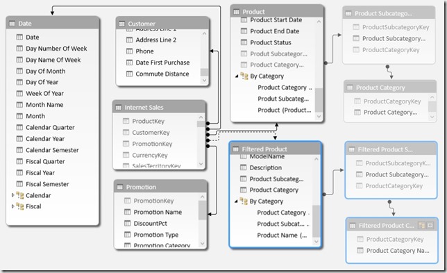
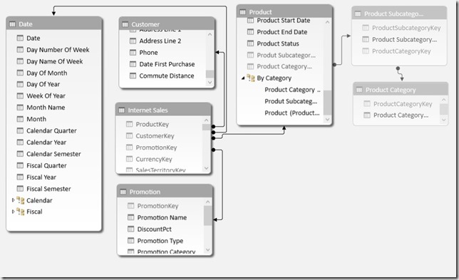
First of all we do not want to modify this model but just extend it so that all previously created measures, calculations and, most important, the reports still work. So the only thing we do is to add our Product-tables again but with a different name. Note that I also added the Subcategory and Category tables in order to allow Basket Analysis also by the Product-Category hierarchy. As we further do not want to break anything we only use an inactive relationship to our ‘Internet Sales’ fact table.

After adding the tables the model looks as follows:Model_New

The next and actually last thing to do is to add the following calculated measure:

Sold in same Order :=
CALCULATE (
COUNTROWS ( ‘Internet Sales’ ),
CALCULATETABLE (
SUMMARIZE (
‘Internet Sales’,
‘Internet Sales’[Sales Order Number]
),
ALL ( ‘Product’ ),
USERELATIONSHIP ( ‘Internet Sales’[ProductKey], ‘Filtered Product’[ProductKey] )
)
)

(formatted using DAX Formatter)

The inner CALCULATETABLE returns a list/table of all [Sales Order Numbers] where a ‘Filtered Product’ was sold and uses this table to extend the filter on the ‘Internet Sales’ table. It is also important to use ALL(‘Product’) here otherwise we would have two filters on the same column ([ProductKey]) which would always result in an empty table. Doing a COUNTROWS finally returns all for all baskets where the filtered product was sold.
We could also change ‘Internet Sales'[Sales Order Number] to ‘Internet Sales'[CustomerKey] in order to analyze what other customers bought also in different baskets (This was done for Example 3). The whole SUMMARIZE-function could also be replaced by VALUES(‘Internet Sales'[Sales Order Number]). I used SUMMARIZE here as I had better experiences with it in terms of performance in the past, though, this may depend on your data. The calculation itself also works with all kind of columns and hierarchies, regardless whether its from table ‘Product’, ‘Filtered Product’, or any other table!

So what can we finally do with this neat formula?

1) Classic Basket Analysis – “Others also bought …”:
Result_ClassicBasketAnalysis

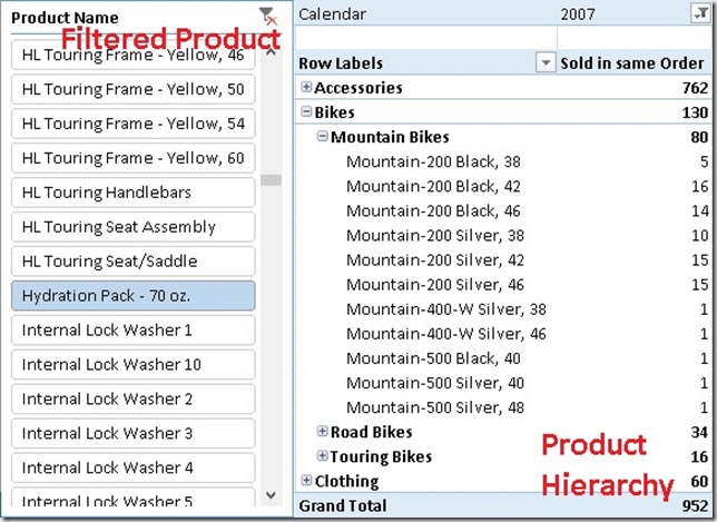
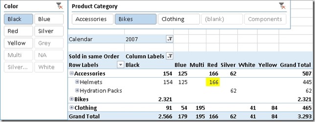
As we can see Hydration Packs are more often sold together with Mountain Bikes opposed to Road Bikes and Touring Bikes. We could also use a slicer on ‘Filtered Product Subcategory’=”Accessories” in order to see how often Accessories are sold together with other products. You may analyze by Color and Product Category:
Result_ByColor
As we can see people that buy black bikes are more likely to buy red helmets than blue helmets.

2) Basket Analysis Matrix:
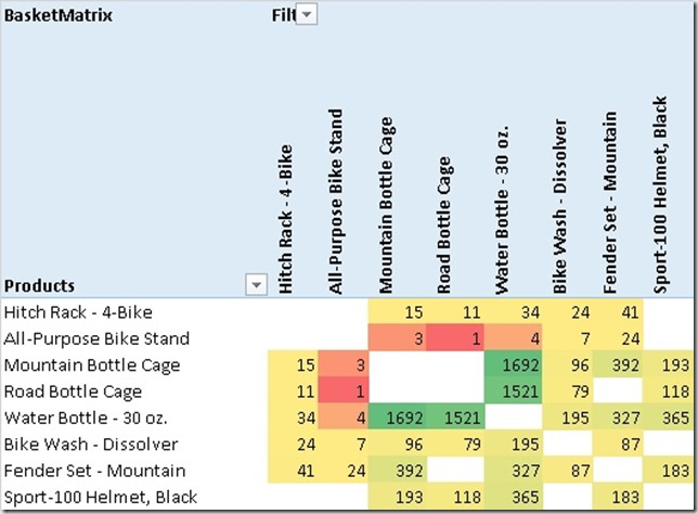
What may also be important for us is which products are sold together the most often? This can be achieved by pulling ‘Product’ on rows and ‘Filtered Product’ on columns. By further applying conditional formatting we can identify correlations pretty easy:
Result_BasketMatrix
Water Bottles are very often sold together with Bottle Cages – well, not really a surprise. Again, you can also use all kind of hierarchies here for your analysis.
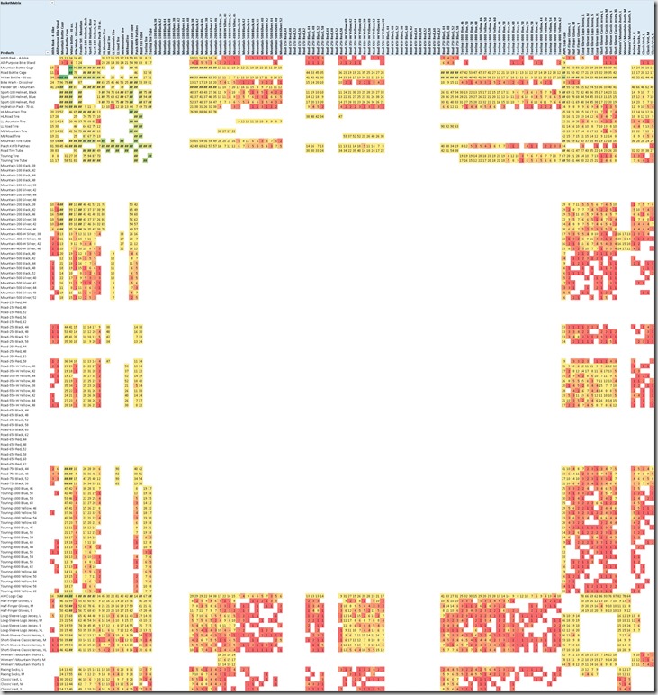
This is what the whole matrix looks like:
Result_BasketMatrixFull
The big blank section in the middle are our Bikes. This tells us that there is no customer that bought two bikes in the same order/basket.

For this analysis I used an extended version of the calculation above to filter out values where ‘Product’ = ‘Filtered Product’ as of course every product is sold within its own basket:

BasketMatrix :=
IF (
MIN ( ‘Product’[ProductKey] )
<> MIN ( ‘Filtered Product’[ProductKey] ),
[Sold in same Order]
)

3) Find Customers that have not bough a common product yet
As we now know from the above analysis which products are very often bought together we can also analyze which customers do not fall in this pattern – e.g. customers who have bough a Water Bottle but have not bought a Bottle Cage yet. Again we can extend our base-calculation to achieve this:

Not Sold to same Customer :=
IF (
NOT ( ISBLANK ( [Sum SA] ) ) && NOT ( [Sold to same Customer] ),
“Not Sold Yet”
)

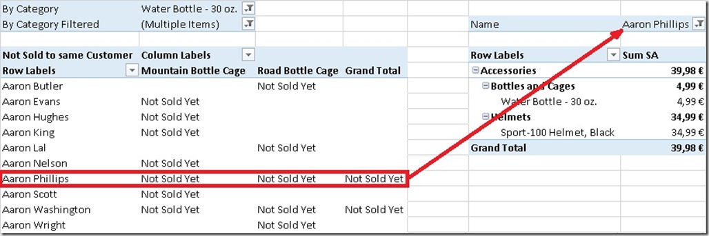
The first part checks if the selected ‘Product’ was sold to the customer at all and the second part checks if the ‘Filtered Product’ was not sold to the customer yet. In that case we return “Not Sold Yet”, and otherwise  BLANK() which is the default if the third parameter is omitted. That’s the result:
Result_NotSoldToCustomer
Aaron Phillips has bought a Water Bottle but no Mountain Bottle Cage nor a Road Bottle Cage – maybe we should send him some advertisement material on Bottle Cages? Smile


As you can see there are a lot of analyses possible on top of that little measure that we created originally. All work with any kind of grouping or hierarchy that you may have and no change to your data model is necessary, just a little extension.

And that’s it – Basket Analysis made easy using Power Pivot and DAX!

Downloads:

Sample Excel Workbook with all Examples: BasketAnalysis.xlsx
Sample PowerBI Desktop file with all Examples (DAX only, no Visuals): BasketAnalysis.pbix

Universal Quantiles Calculation for PowerPivot using DAX

In my last post I showed a new approach on how to calculate the median in PowerPivot using DAX. In the comments the question was raised whether it is possible to make that calculation universal for all kind of Quantiles like Median, Quartiles, Percentiles, etc. and that’s what this post is about.

Lets analyze the final Median calculation from the last post:

Median SA Months:=CALCULATE([SumSA],
TOPN(
2-MOD([Cnt_Months], 2),
TOPN(
([Cnt_Months] + 1) / 2,
VALUES(‘Date’[Month]),
[SumSA]),
[SumSA],
1))
/
(2-MOD([Cnt_Months], 2))


The Median defines the value in the middle of an ordered set. To get the first half (+1 to handle even and odd sets) of the whole we are using TOPN function:

TOPN(
([Cnt_Months] + 1) / 2,
VALUES(‘Date’[Month]),
[SumSA]),

The important part here is the “divide by 2” to split the set in the middle to start our Median calculation. Instead of dividing by 2 we could also multiply by 0.5 where 0.5 would be the separator for our quantile (in this case the Median). This expression can be made dynamic. For the first Quartile we would use 0.25 for the second Quartile (=Median) we would use 0.5 and for the third Quartile we would use 0.75.

I created a little linked table to demonstrate the dynamic approach:

Quantile SortOrder Percentage
Median 1 0.5000
Quartile 1 401 0.2500
Quartile 2 402 0.5000
Quartile 3 403 0.7500
Sextile 1 601 0.1667
Sextile 2 602 0.3333
Sextile 3 603 0.5000
Sextile 4 604 0.6667
Sextile 5 605 0.8333

We also need to add a calculated measure that returns the percentage-value of the currently selected Quantile:

SelectedQuantile:=IF(
HASONEVALUE(Quantiles[Percentage]),
VALUES(Quantiles[Percentage]))


Now we can change our old Median-calculation to be dynamic by using the measure defined above:

Quantile SA Months:=CALCULATE([SumSA],
TOPN(
2 – MOD([Cnt_Months], 2),
TOPN(
ROUNDUP(([Cnt_Months] + 1) * [SelectedQuantile], 0),
VALUES(‘Date’[Month]),
[SumSA]),
[SumSA],
1))
/
(2 – MOD([Cnt_Months], 2))

We also need to explicitly add ROUNDUP() as “([Cnt_Months] + 1) * [SelectedQuantile]” may return any decimal places whereas the previous divide by 2 could only result in a x.5 which was rounded up automatically. And well, that’s all we need to change in order to make the calculation universal for all different Quantiles! The rest is the same logic that I already described for Median calculation.


Download Final Model (Office 2013!)

Calculating Median in PowerPivot using DAX

I just came across this blog post by Bill Anton where he discusses several approaches to calculated the Median of a given set in T-SQL, MDX and DAX. In the end of his post when it comes to the DAX calculation, he references several post by Marco, Alberto and Javier (post1, post2) that already address that kind of calculation in DAX. But he also claims that non of the solutions is “elegant”. Well, reason enough for me to try it on my own and here is what I came up with. Its up to you to decide whether this solution is more elegant than the others or not 🙂

In general, the median calculation always varies depending on the number of items and whether this number is even or odd.
For an even population the median is the mean of the values in the middle:
the median of {3, 5, 7, 9} is is (5 + 7)/2 = 6
For an odd population, the median is the value in the middle:
the median of {3, 5, 9} is 5

In both cases the values have to be ordered before the calculation. Note that it does not make a difference whether the values are sorted in ascending or descending order.

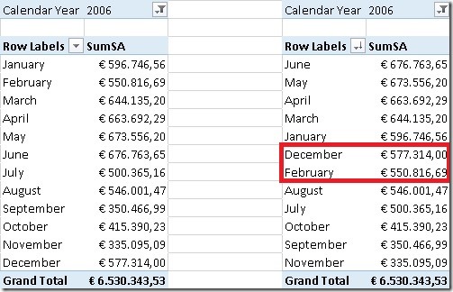
OrderedValues

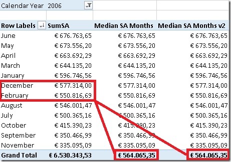
In this example, our set contains 12 items (=months) so we have to find the 2 items in the middle of the ordered set – December and February – and calculate the mean.

So, how can we address this problem using DAX? Most of the posts I mentioned above use some kind of combination of ranking – RANKX() – and filtering – FILTER(). For my approach I will use none of these but use TOPN instead (yes, I really like that function as you probably know if you followed my blog for some time).

In this special case, TOPN() can do both, ranking and filtering for us. But first of all we need to know how many items exist in our set:

Cnt_Months:=DISTINCTCOUNT(‘Date’[Month])


This value will be subsequently used in our next calculations.

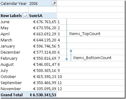
To find the value(s) in the middle I use TOPN() twice, first to get the first half of the items (similar to TopCount) and then a second time to get the last values that we need for our median calculation (similar to BottomCount):

TopBottom

As the median calculation is different for even and odd sets, this also has to be considered in our calculation. For both calculations MOD()-function is used to distinguish both cases:

Items_TopCount:=IF(MOD([Cnt_Months],2) = 0,
([Cnt_Months] / 2) + 1,
([Cnt_Months] + 1) / 2)

For an even number of items (e.g. 12) we simply divide the count of items by 2 and add 1 which gives us a (12 / 2) + 1 = 7 for our sample.
For an odd number of items (e.g. 5) we first add 1 to our count of items and then divide by 2 which gives us (5 + 1) / 2 = 3

Items_BottomCount:=IF(MOD([Cnt_Months],2) = 0, 2, 1)

For an even number of items we have to consider the last 2 values whereas for an odd number of items we only have to consider the last value.


These calculations are then used in our median calculation:

Median SA Months:=CALCULATE([SumSA],
TOPN(
[Items_BottomCount],
TOPN(
[Items_TopCount],
VALUES(‘Date’[Month]),
[SumSA]),
[SumSA] * -1))
/
[Items_BottomCount]

As DAX has no built-in BOTTOMN()-function, we need to “abuse” the TOPN() function and multiply the OrderBy-value by “–1” to get the BOTTOMN() functionality. As you can see most of the logic is already handled by our [Items_TopCount] and [Items_BottomCount] measures and this pattern can be reused very easily.


Of course all these calculations can also be combined and the use of IF() can be avoided:

Median SA Months v2:=CALCULATE([SumSA],
TOPN(
2 – MOD([Cnt_Months], 2),
TOPN(
([Cnt_Months] + 1) / 2,
VALUES(‘Date’[Month]),
[SumSA]),
[SumSA] * -1))
/
(2 – MOD([Cnt_Months], 2))

Note: for an even population ([Cnt_Months] + 1) / 2 returns X.5 which is automatically rounded up when it is used in a function that expects a whole number. In our example this is what happens: (12 + 1) / 2 = 6.5 –> 7

These are the final results:

FinalResults


Additional content:

We could also use AVERAGEX() to calculate our median but I think that it is some kind of overhead to use AVERAGEX() just to divide by “1” or “2” depending on the number of items that our TOPN-functions return:

Median SA Months AvgX:=AVERAGEX(
TOPN(
2-MOD([Cnt_Months], 2),
TOPN(
([Cnt_Months] +1) / 2,
VALUES(‘Date’[Month]),
[SumSA]),
[SumSA] * -1),
[SumSA])


As you can see there are various approaches to calculate the median, its up to you which on you like most. I have not tested any of them in terms of performance over bigger sets – this may be topic for an upcoming post.


Download Final Model (Office 2013!)

Another Post about Calculating New and Returning Customers – Part 2

In my previous post I showed a new approach on how to calculate new (and returning) customers in PowerPivot/tabular using DAX. We ended up with a solution where we added the customers first order date as a calculated column to our customer-table. This column was then linked to our date-table with an inactive relationship. The final calculation used USERELATIONSHIP() to make use of this relationship as follows:

New Customers:=CALCULATE(
COUNTROWS(Customer),
USERELATIONSHIP(Customer[FirstOrderDate], ‘Date’[Date]))

This calculation performs really well as it does not have to touch the fact-table to get the count of new customers. And this is also the issue with the calculation as other filters are not reflected in the calculation:

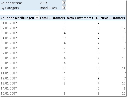
Issue_Old_vs_New

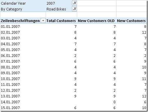
Take row 2 as an example: we have 8 “Total Customers” of which 12 are “New Customers”. Obviously an error in the calculation. The PivotTable is filtered to Category=”Road Bikes” and we have 8 customers on the 2nd of February that bought a road bike. The “New Customers” calculation on the other hand is not related to the Subcategory and shows 12 as in total there were 12 new customers for all products.


To get our calculation working also with other filters we have to somehow relate it to our fact-table. So far we calculated the customers first order date only in the customer table. The customers first order may be related to several fact-rows, e.g. one row for each product the customer bought. Our “New Customers” calculation should only include customers that are active considering also all other filters.

To identify a customers first order in our fact-table we can again use a calculated column and also re-use our previous calculated column in our Customer-table that holds the customers first order date:

=NOT(
ISBLANK(
LOOKUPVALUE(
Customer[CustomerKey],
[CustomerKey],
Customer[FirstOrderDate],
[Order Date]
)))

This returns True for all fact-rows associated with a customers first order and False for all other rows.

The final “New Customers v2” calculation is quite simple then – in addition to the active filters we add a further filter to only select rows that are associated to a customers first order:

New Customers v2:=CALCULATE(
[Total Customers],
‘Internet Sales’[IsCustomersFirstOrder] = TRUE())


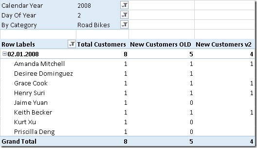
And this are the results:

Final_Old_vs_NewV2

As you can see there are still differences between “New Customers OLD” and “New Customers v2”. But is this really a problem with the new calculation? Lets analyze the issue taking customer “Desiree Dominguez” where we encounter the first difference as an example:

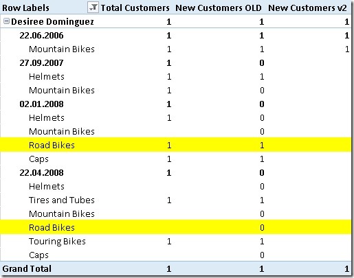
Issue_Analyzed

“Desiree Dominguez” had her first order on the 22th of June in 2006. So she is actually no “new customer” in 2008. The reason why the old calculation counts her as “new customer” is that it was the first time that she bought a product of subcategory “Road Bikes”. Whether this is correct or not is up to your business definition of a “new customer”. According to my experience it is more likely that “Desiree Dominguez” is not counted as a new customer in 2008 and so the “New Customer v2” actually returns the more accurate results.


Additional stuff:

An other option for this calculation is to rank the [Order Date] or [Sales Order Number] for each customer within the fact-table using the calculation below:

=RANKX(
FILTER(
ALL(‘Internet Sales’),
[CustomerKey] = EARLIER([CustomerKey])),
[Order Date],
[Order Date],
1,
DENSE
)

[Order Date] could be replaced by [Sales Order Number]. This makes sense if a customer can have multiple orders per day and you also want to distinguish further by [Sales Order Number]. The new field would also allow new analysis. For example the increase/decrease in sales from the second order compared to the first order and so on.

The “New Customer” calculation in this case would still be similar. We just have to filter on the new calculated column instead:

New Customers v3:=CALCULATE(
[Total Customers],
‘Internet Sales’[CustomersOrderNr] = 1)


Download Final Model (Office 2013!)


The multidimensional model:

The whole logic of extending the fact-table to identify rows that can be associated with a customers first order can also be used in a multidimensional model. Once we prepared the fact-table accordingly the calculations are quite easy. The biggest issues here does not reside in the multidimensional model itself but in the ETL/relational layer as this kind of operation can be quite complex – or better say time-consuming in terms of ETL time.

At this point I will not focus on the necessary ETL steps but start with an already prepared fact-table and highlight the extensions that have to be made in the multidimensional model. The fact-table already got extended by a new column called [IsCustomersFirstOrder] similar to the one we created in tabular using a DAX calculated column. It has a value of 1 for rows associated with a customers first order and 0 for all other rows.

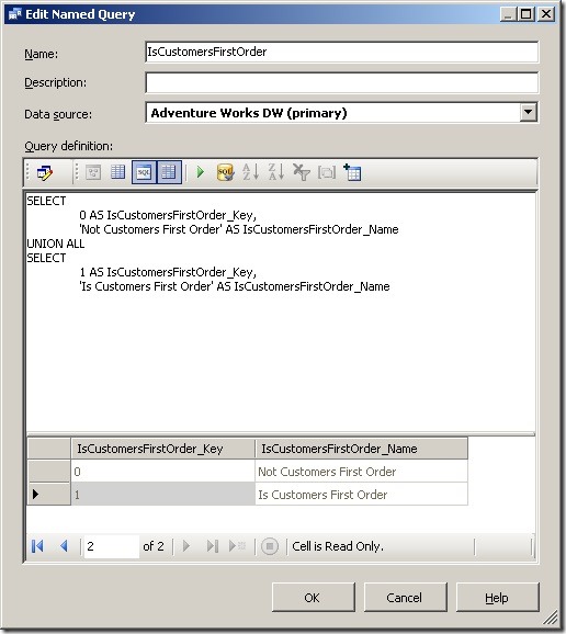
The next thing we have to do is to create a new table in our DSV to base our new dimension on. For simplicity I used this named query:

MD_NamedQuery_Dim

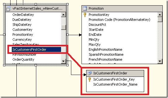
This table is then joined to the new fact-table:

MD_DSV

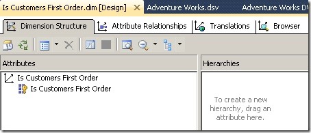
The new dimension is quite simple as it only contains one attribute:

MD_Dimension

You may hide the whole dimension in the end as it may only be used to calculate our “new customers” and nowhere else and may only confuse the end-user.


Once we have added the dimension also to our cube we can create a new calculated measure to calculate our “new customers” as follows:

CREATE MEMBER CURRENTCUBE.[Measures].[New Customers] AS (
[Measures].[Customer Count],
[Is Customers First Order].[Is Customers First Order].&[1]
), ASSOCIATED_MEASURE_GROUP = ‘Internet Customers’
, FORMAT_STRING = ‘#,##0’;

The calculation is based on the existing [Customer Count]-measure which uses DistinctCount-aggregation. Similar to DAX with just extend the calculation by further limiting the cube-space where “Is customers First Order” = 1.

This approach also allows you to create aggregations if necessary to further improve performance. So this is probably also the best way in terms of query-performance to calculate the count of new customers in a multidimensional model.

Another Post about Calculating New and Returning Customers

I know, this topic has already been addressed by quite a lot of people. Chris Webb blogged about it here(PowerPivot/DAX) and here(SSAS/MDX), Javier Guillén here, Alberto Ferrari mentions it in his video here and also PowerPivotPro blogged about it here. Still I think that there are some more things to say about it. In this post I will review the whole problem and come up with a new approach on how to solve this issue for both, tabular and multidimensional models with the best possible performance I could think of (hope I am not exaggerating here  🙂 )

OK, lets face the problem of calculating new customers first and define what a new customer for a given period actually is:

A new customer in Period X is a customer that has sales in Period X but did not have any other sales ever before. If Period X spans several smaller time periods
(e.g. Period X=January contains 31 days) then there must not be any sales before the earliest smaller time period (before 1st of January) for this customer to be counted as a new customer.

According to this definition the common approach can be divided into 2 steps:
1) find all customers that have sales till the last day in the selected period
2) subtract the number of customers that have sales till the day before the first day in the
selected period


First of all we need to create a measure that calculates our distinct customers.
For tabular it may be a simple calculated measure on your fact-table:

Total Customers:=DISTINCTCOUNT(‘Internet Sales’[CustomerKey])

For multidimensional models it should be a physical distinct count measure in your fact-table, ideally in a separate measure group.

How to solve 1) in tabular models

This is also straight forward as DAX has built-in functions that can do aggregation from the beginning of time. We use MAX(‘Date’[Date]) to get the last day in the current filter context:

Customers Till Now:=CALCULATE(
[Total Customers],
DATESBETWEEN(
‘Date’[Date],
BLANK(),
MAX(‘Date’[Date])))


How to solve 2) in tabular models

This is actually the same calculation as above, we only use MIN to get the first day in the current filter context and also subtractt “1” to get the day before the first day.

Previous Customers:=CALCULATE(
[Total Customers],
DATESBETWEEN(
‘Date’[Date],
BLANK(),
MIN(‘Date’[Date])-1))


To calculate our new customers we can simply subtract those two values:

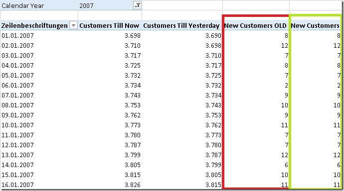
New Customers OLD:=[Customers Till Now]-[Previous Customers]


How to solve 1) + 2) in multidimensional models

Please refer to Chris Webb’s blog here. The solution is pure MDX and is based on a combination of the range-operator “{null:[Date].[Calendar].currentmember}”, NONEMPTY() and COUNT().


Well, so far nothing new.


So lets describe the solution that I came up with. It is based on a different approach. To make the approach easily understandable, we have to rephrase the answer to our original question “What are new customers”?”:

A new customer in Period X is a customer that has his first sales in Period X.

According to this new definition we again have 2 steps:
1) Find the first date with sales for each customer
2) count the customers that had their first sales in the selected period

I will focus on tabular models. For multidimensional models most of the following steps have to be solved during ETL.


How to solve 1) in tabular models

This is pretty easy, we can simply create a calculated column in our Customer-table and get the first date on which the customer had sales:

=CALCULATE(MIN(‘Internet Sales’[Order Date]))


How to solve 2) in tabular models

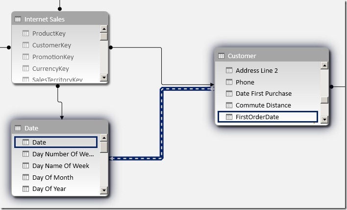
The above create calculated column allows us to relate our ‘Date’-table directly to our ‘Customer’-table. As there is already an existing relationship between those tables via ‘Internet Sales’ we have to create an inactive relationship at this point:

Customer_Date_Relationship

Using this new relationship we can very easy calculate customers that had their first sales in the selected period:

New Customers:=CALCULATE(
COUNTROWS(Customer),
USERELATIONSHIP(Customer[FirstOrderDate], ‘Date’[Date]))


Pretty neat, isn’t it?
We can use COUNTROWS() opposed to a distinct count measure as our ‘Customer’-table only contains unique customers – so we can count each row in the current filter context.
Another nice thing is that we do not have to use any Time-Intelligence function like DATESBETWEEN which are usually resolved using FILTER that would iterate over the whole table. Further it also works with all columns of our ‘Date’-table, no matter whether it is [Calendar Year], [Fiscal Semester] or [Day Name of Week]. (Have you ever wondered how many new customers you acquired on Tuesdays? 🙂 )   And finally, using USERELATIONSHIP allows us to use the full power of xVelocity as native relationships are resolved there.


The results are of course the same as for [New Customers OLD]:

Result_Old_vs_New


Though, there are still some issues with this calculation if there are filters on other tables:

Issue_Old_vs_New

As you can see, our new [New Customers] measure does not work in this situation as it is only related to our ‘Date’-table but not to ‘Product’.

I will address this issue in a follow-up post where I will also show how the final solution can be used for multidimensional models – Stay tuned!

Download Final Model (Office 2013!)


UPDATE: Part2 can be found here

Dynamic ABC Analysis in PowerPivot using DAX

An ABC Analysis is a very common requirement for for business users. It classifies e.g. Items, Products or Customers into groups based on their sales and how much impact they had on the cumulated overall sales. This is done in several steps.

I just published a new version of the Dynamic ABC Analysis at www.daxpatterns.com. The article can be found here.


1) Order products by their sales in descending order
2) Cumulate the sales beginning with the best selling product till the current product
3) Calculate the percentage of the cumulated sales vs. total sales
4) Assign a Class according to the cumulated percentage

Marco Russo already blogged about this here. He does the classification in a calculated column based on the overall sales of each product. As calculated columns are processed when the data is loaded, this is not dynamic in terms of your filters that you may apply in the final report. If, for example, a customer was within Class A regarding total sales but had no sales last year then a report for last year that uses this classification may give you misleading results.

In this blog I will show how to do this kind of calculation on-the-fly always in the context of the current filters. I am using Adventure Works DW 2008 R2 (download) as my sample data and create a dynamic ABC analysis of the products.

The first thing we notice is that our product table is a slowly changing dimension of type 2 and there are several entries for the same product as every change is traced in the same table.

SCD2Table

So we want to do our classification on the ProductAlternateKey (=Business Key) column instead of our ProductKey (=Surrogate Key) column.

First we have to create a ranking of our products:

Rank CurrentProducts:=IF(HASONEVALUE(DimProduct[ProductAlternateKey]),
IF(NOT(ISBLANK([SUM SA])),
RANKX(
CALCULATETABLE(
VALUES(DimProduct[ProductAlternateKey]),
ALL(DimProduct[ProductAlternateKey])),
[SUM SA])))

Check if there is only one product in the current context and that this product also has sales. If this is the case we calculate our rank. We need to do the CALCULATETABLE to do the ranking within the currently applied filters on other columns of the DimProduct-table e.g. if a filter is applied to DimProduct[ProductSubcategoryKey] we want to see our ranking within that selected Subcategory and not against all Products.

I also created a measure [SUM SA] just to simplify the following expressions:

SUM SA:=SUM(FactInternetSales[SalesAmount])


The second step is to create a running total starting with the best-selling product/the product with the lowest rank:

CumSA CurrentProducts:=SUMX(
TOPN(
[Rank CurrentProducts],
CALCULATETABLE(
VALUES(DimProduct[ProductAlternateKey]),
ALL(DimProduct[ProductAlternateKey])),
[SUM SA]),
[SUM SA])

We use a combination of SUMX() and TOPN() here. TOPN() returns the top products ordered by [SUM SA]. Further we use our previously calculated rank to only get the products that have the same or more sales than the current product. For example if the current product has rank 3 we sum up the top 3 products to get our cumulated sum (=sum of the first 3 products) for this product. Again we need to use CALCULATETABLE() to retain other filters on the DimProduct-table.


The third step is pretty easy – we need to calculate percentage of the cumulated sales vs. the total sales:

CumSA% CurrentProducts:=
[CumSA CurrentProducts]
/
CALCULATE([SUM SA], ALL(DimProduct[ProductAlternateKey]))

This calculation is straight forward and should not need any further explanation.

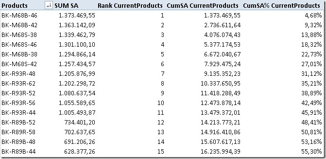
The result of those calculations can be seen here:

Theory


To do our final classification we have to extend our model with a new table that holds our classes and their border-values:

Class LowerBoundary UpperBoundary
A 0 0.7
B 0.7 0.9
C 0.9 1

Class A should contain products which’s cumulated sales are between 0 and 0.7 – between 0% and 70%.
Class B should contain products which’s cumulated sales are between 0.7 and 0.9 – between 70% and 90%.
etc.

(This table can later be extended to support any number of classes and any boundaries between 0% and 100%.)

To get the boundaries of the selected class we create two measures that are later used in our final calculation:

MinLowerBoundary:=MIN([LowerBoundary])
MaxUpperBoundary:=MAX([UpperBoundary])


Our final calculation looks like this:

SA Classified Current:=IF(NOT(ISCROSSFILTERED(Classification[Class])),
[SUM SA],
CALCULATE(
[SUM SA],
FILTER(
VALUES(DimProduct[ProductAlternateKey]),
[MinLowerBoundary] < [CumSA% CurrentProducts]
&& [CumSA% CurrentProducts] <= [MaxUpperBoundary])))

If our Classification-table is not filtered, we just show our [SUM SA]-measure. Otherwise we extend the filter on our DimProduct[ProductAlternateKey] using our classification filtering out all products that do not fall within the borders of the currently selected class.

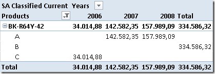
This measure allows us to see the changes of the classification of a specific product e.g. over time:

FinalResults_1

In 2006 our selected product was in Class C. For 2007 and 2008 it improved and is now in Class A. Still, overall it resides in Class B.

We may also analyze the impact of our promotions on the sales of our classified products:

FinalResults_2

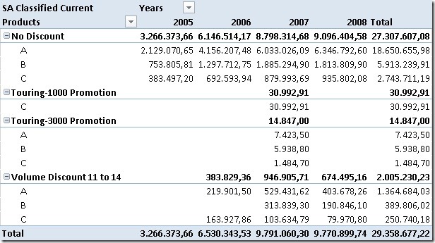
Our Promotion “Touring-1000 Promotion” only had impact on products in Class C so we may consider to stop that promotion and invest more into the other promotions that affect all classes.


The classification can be used everywhere you need it – in the filter, on rows or on columns, even slicers work. The only drawback is that the on-the-fly calculation can take quite some time. If I find some time in the future i may try to further tune them and update this blog-post.


The example workbook can be downloaded here:

Though it is already in Office 2013 format an may not be opened with any previous versions of Excel/PowerPivot.
It also includes a second set of calculations that use the same logic as described above but does all the calculations without retaining any filters on the DimProducts-table. This allows you to filter on Class “A” and ProductSubcategory “Bike Racks” realizing that “Bike Racks” are not a Class “A” product or to see which Subcategories or Categories actually contain Class A, B or C products!