Running Local R Scripts in Power BI

One of the coolest features of Power BI is that I integrates very well with other tools and also offers a lot of interfaces which can be used to extend this capabilities even further. One of those is the R Integration which allows you to run R code from within Power BI. R scripts can either be used as a data source or for visualizing your data. In this post I will focus on the data source component and show how you can use a locally stored R script and execute it directly in Power BI. Compared to the native approach where you need to embed the R code in the Power BI file, this has several advantages:

  • Develop R script in familiar external tool like RStudio
  • Integration with Source Control
  • Leverage Power BI for publishing and visualizing results

Out of the box Power BI only supplies one function to call R scripts as a data source which is R.Execute(text). Usually, when you use the wizard, it simply passes your R script as a hardcoded value to this function. Knowing the power of Power BI and its scripting language M for data integration made me think – “Hey, as R scripts are just text files and Power BI can read text files, I could also dynamically read any R script and execute it!”

Well, turns out to be true! So I created a little M function where I pass in the file-path of an existing R script and which returns a table of data frames which are created during the execution of the script. Those can then be used like any other data sets/tables within Power BI:
Power_BI_R_DataSource_dynamic_local_script

And here is the corresponding M code for the Power Query function:
(Thanks also to Imke Feldmann for simplifying my original code to the readable one below)

  1. let
  2.     LoadLocalRScript = (file_path as text) as table =>
  3. let
  4.     Source = Csv.Document(File.Contents(file_path),[Delimiter=#(lf), Columns=1, Encoding=1252, QuoteStyle=QuoteStyle.None]),
  5.     RScript =  Text.Combine(Source[Column1], "#(lf)"),
  6.     output = R.Execute(RScript)
  7. in
  8.     output
  9. in
  10.     LoadLocalRScript

First we read the R script like any other regular CSV file but we use line-feed (“#(lf)”) as delimiter. So we get a table with one column and one row for each line of our original R script.
Then we use Text.Combine() on our column to transform the single lines back into one long text resembling our original R script. This text can the be passed to the R.Execute() function to return the list of R data frames created during the execution of the script.

And that’s it! Any further steps are similar to using any regular R script which is embedded in Power BI so it is up to you on how you proceed from here. Just one thing you need to keep in mind is that changing the local R script might break the Power BI load if you changed or deleted any data frames which are referenced in Power BI later on.

One issues that I came across during my tests is that this approach does not work with scheduled refreshes in the Power BI Web Service via the Personal Gateway. The first reason for this is that it is currently not possible to use scheduled refresh if custom functions are involved. Even if you can work around this issue pretty easily by using the code from above directly in Power Query I still ran into issues with different privacy levels for the location of the R script and the R.Execute() function. But I will investigate into those issues and update this blog post accordingly (see UPDATE below).
For the future I hope that is fixed by Microsoft and Power BI allows you to execute remote scripts natively – but until then, this approach worked quite well for me.

UPDATE:
To make the refresh via the Personal Gateway work you have to enable “FastCombine”. How to do this is described in more detail here: Turn on FastCombine for Personal Gateway.

In case you are interested in more details on this approach, I am speaking at TugaIT in Lisbon, Portugal this Friday (20th of May 2016) about “Power BI for the Data Scientist” where I will cover this and lots of other interesting topics about the daily work of a data scientist and how PowerBI can used to ease them.

Downloads:
Power BI Workbook: Load_Local_R_Script_wFunction.pbix
Sample R Script: Sample_R_Script.r

Dynamic ABC Analysis in Power Pivot using DAX – Part 2

Almost two years ago I published the first version of an Dynamic ABC Analysis in Power Pivot and by now it is the post with the most comments among all my blog posts. This has two reason:
1) the formula was quite complex and not easy to understand or implement
2) the performance was not really great with bigger datasets

When the first of those comments flew in, I started investigating into a new, advanced formula. At about the same time Marco Russo and Alberto Ferrari published their ABC Classification pattern – a static version using calculated columns – at www.daxpatterns.com. When I had my first dynamic version ready I sent it to Marco and Alberto and asked if they are interested in the pattern and if I can publish it on their website. Long story short – this week the new pattern was released and can now be found here:

ABC Classification – Dynamic

It got some major performance improvements and was also designed towards reusability with other models. The article also contains some detailed explanations how the formula actually works but its still very hard DAX which will take some time to be fully understood. The pattern also features some extended versions to address more specific requirements but I think its best to just read the article on your own.

Hope you enjoy it!

Dynamic ABC Analysis in PowerPivot using DAX

An ABC Analysis is a very common requirement for for business users. It classifies e.g. Items, Products or Customers into groups based on their sales and how much impact they had on the cumulated overall sales. This is done in several steps.

I just published a new version of the Dynamic ABC Analysis at www.daxpatterns.com. The article can be found here.


1) Order products by their sales in descending order
2) Cumulate the sales beginning with the best selling product till the current product
3) Calculate the percentage of the cumulated sales vs. total sales
4) Assign a Class according to the cumulated percentage

Marco Russo already blogged about this here. He does the classification in a calculated column based on the overall sales of each product. As calculated columns are processed when the data is loaded, this is not dynamic in terms of your filters that you may apply in the final report. If, for example, a customer was within Class A regarding total sales but had no sales last year then a report for last year that uses this classification may give you misleading results.

In this blog I will show how to do this kind of calculation on-the-fly always in the context of the current filters. I am using Adventure Works DW 2008 R2 (download) as my sample data and create a dynamic ABC analysis of the products.

The first thing we notice is that our product table is a slowly changing dimension of type 2 and there are several entries for the same product as every change is traced in the same table.

SCD2Table

So we want to do our classification on the ProductAlternateKey (=Business Key) column instead of our ProductKey (=Surrogate Key) column.

First we have to create a ranking of our products:

Rank CurrentProducts:=IF(HASONEVALUE(DimProduct[ProductAlternateKey]),
IF(NOT(ISBLANK([SUM SA])),
RANKX(
CALCULATETABLE(
VALUES(DimProduct[ProductAlternateKey]),
ALL(DimProduct[ProductAlternateKey])),
[SUM SA])))

Check if there is only one product in the current context and that this product also has sales. If this is the case we calculate our rank. We need to do the CALCULATETABLE to do the ranking within the currently applied filters on other columns of the DimProduct-table e.g. if a filter is applied to DimProduct[ProductSubcategoryKey] we want to see our ranking within that selected Subcategory and not against all Products.

I also created a measure [SUM SA] just to simplify the following expressions:

SUM SA:=SUM(FactInternetSales[SalesAmount])


The second step is to create a running total starting with the best-selling product/the product with the lowest rank:

CumSA CurrentProducts:=SUMX(
TOPN(
[Rank CurrentProducts],
CALCULATETABLE(
VALUES(DimProduct[ProductAlternateKey]),
ALL(DimProduct[ProductAlternateKey])),
[SUM SA]),
[SUM SA])

We use a combination of SUMX() and TOPN() here. TOPN() returns the top products ordered by [SUM SA]. Further we use our previously calculated rank to only get the products that have the same or more sales than the current product. For example if the current product has rank 3 we sum up the top 3 products to get our cumulated sum (=sum of the first 3 products) for this product. Again we need to use CALCULATETABLE() to retain other filters on the DimProduct-table.


The third step is pretty easy – we need to calculate percentage of the cumulated sales vs. the total sales:

CumSA% CurrentProducts:=
[CumSA CurrentProducts]
/
CALCULATE([SUM SA], ALL(DimProduct[ProductAlternateKey]))

This calculation is straight forward and should not need any further explanation.

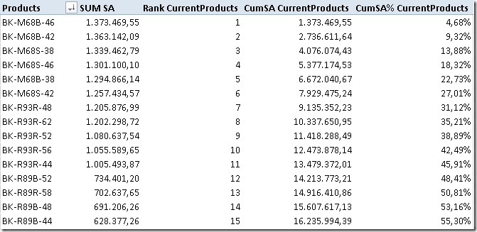
The result of those calculations can be seen here:

Theory


To do our final classification we have to extend our model with a new table that holds our classes and their border-values:

Class LowerBoundary UpperBoundary
A 0 0.7
B 0.7 0.9
C 0.9 1

Class A should contain products which’s cumulated sales are between 0 and 0.7 – between 0% and 70%.
Class B should contain products which’s cumulated sales are between 0.7 and 0.9 – between 70% and 90%.
etc.

(This table can later be extended to support any number of classes and any boundaries between 0% and 100%.)

To get the boundaries of the selected class we create two measures that are later used in our final calculation:

MinLowerBoundary:=MIN([LowerBoundary])
MaxUpperBoundary:=MAX([UpperBoundary])


Our final calculation looks like this:

SA Classified Current:=IF(NOT(ISCROSSFILTERED(Classification[Class])),
[SUM SA],
CALCULATE(
[SUM SA],
FILTER(
VALUES(DimProduct[ProductAlternateKey]),
[MinLowerBoundary] < [CumSA% CurrentProducts]
&& [CumSA% CurrentProducts] <= [MaxUpperBoundary])))

If our Classification-table is not filtered, we just show our [SUM SA]-measure. Otherwise we extend the filter on our DimProduct[ProductAlternateKey] using our classification filtering out all products that do not fall within the borders of the currently selected class.

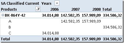
This measure allows us to see the changes of the classification of a specific product e.g. over time:

FinalResults_1

In 2006 our selected product was in Class C. For 2007 and 2008 it improved and is now in Class A. Still, overall it resides in Class B.

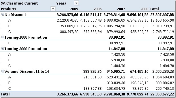
We may also analyze the impact of our promotions on the sales of our classified products:

FinalResults_2

Our Promotion “Touring-1000 Promotion” only had impact on products in Class C so we may consider to stop that promotion and invest more into the other promotions that affect all classes.


The classification can be used everywhere you need it – in the filter, on rows or on columns, even slicers work. The only drawback is that the on-the-fly calculation can take quite some time. If I find some time in the future i may try to further tune them and update this blog-post.


The example workbook can be downloaded here:

Though it is already in Office 2013 format an may not be opened with any previous versions of Excel/PowerPivot.
It also includes a second set of calculations that use the same logic as described above but does all the calculations without retaining any filters on the DimProducts-table. This allows you to filter on Class “A” and ProductSubcategory “Bike Racks” realizing that “Bike Racks” are not a Class “A” product or to see which Subcategories or Categories actually contain Class A, B or C products!