Consolidation and Intercompany Elimination with parallel hierarchies

In my last post I described and approach on how to calculate consolidated values (adjusted by intercompany eliminations) using PowerPivot and DAX. In this post I will extend this technique so it can also be used with parallel hierarchies as this is also very common in financial applications.

Switching from a single hierarchy to multiple parallel hierarchies has several drawbacks for tabular models:
1) business keys cannot be used to build the PC-hierarchy as they are not unique anymore
2) artificial keys and parent-keys are required
3) as business keys are not unique anymore, we also cannot create a relationship between facts and our dimension
4) PowerPivot tables do not support “UNION” to load several single hierarchies and combine them

All the issues described above have to be handled before the hierarchies can be loaded into PowerPivot. This is usually done in a relational database but this will not be covered in this post.

For simplicity I created a table in Excel that already has the correct format:

IDParentIDSenderIDName
1 TOTMy Whole Company by Region
21EUROPEEurope
32GERGermany Company
42FRFrench Company
51NANorth America
65USAUS Company
75CANCanadian Company
-99 EXTERNALEXTERNAL
8 TOT_2My Whole Company Legal View
98JVJoint Ventures
109FRFrench Company
119USAUS Company
128HOLDMy cool Holding
1312GERGermany Company
1412CANCanadian Company

We have 2 parallel hierarchies – “My Whole Company by Region” and “My Whole Company Legal View”. In PowerPivot this looks like this:

Each Company can be assigned to different nodes in every hierarchy.

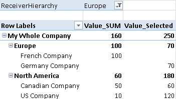
As I already noted above, the SenderIDs are not unique anymore, and therefore we cannot create a relationship to our fact-table. So we have to handle this in our calculation. The approach is similar to handling SCD2 dimensions in PowerPivot what I described in previous posts (Part1 and Part2). We use CONTAINS-function to filter our fact-table based on the currently active SenderIDs in the dimension-table:

Actually this is the only difference in the calculation when we are dealing with multiple parallel hierarches. The other calculations are the same with the only difference that we have to use [Value_Sender] instead of [Value_SUM]:

and

As you can see this approach also works very well with multiple hierarchies. In the end we get the desired results:

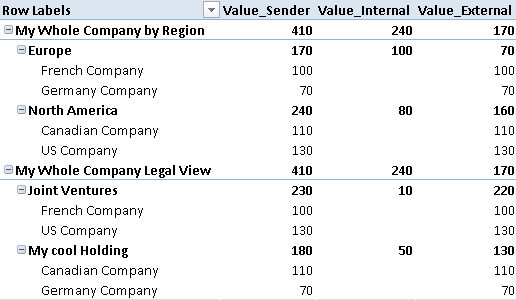
Taking a look at “My cool Holding” we see that a value of 50 is eliminated as there have been sales from CAN to GER. On top-level of the hierarchy we see the same values being eliminated (170) as both hierarchies contain the same companies and therefore only sales to EXTERNAL can summed up to get the correct value.

As this technique operates on leaf-level it works with all possible hierarchies regardless of how many companies are assigned to which node or how deep the hierarchies are!

(Just to compare the values from above – the fact-table is the same as in the previous post: )

SenderIDReceiverIDValue
FRGER100
CANGER50
GEREXTERNAL70
USACAN30
USAFR10
USAEXTERNAL90
CANUSA50
CANEXTERNAL10

Consolidation and Intercompany Elimination made easy using PowerPivot and DAX

In my past years as a consultant for Microsoft BI I had to deal with financial models quite a lot. They are usually small in size but very complex in terms of calculations like currency conversion, margin-calculations, benchmarks and so on. Another topic I came across very frequently was consolidation and intercompany eliminations. Recently I had to deal with this topic again and thought of how this could be solved in PowerPivot/DAX.

First of all a little background information on what consolidation and intercompany eliminations are. In bigger companies with several subsidiaries those subsidiaries are usually structured in some way – e.g. by legal entity, by country etc..

Here is a little example of a corporate group called “My Whole Company” with subsidiaries in Germany, France, USA and Canada, structured by geography:

These companies also make business with each other and also with external customers. The French Company and the Canadian Company sell something to the Germany Company, US Company sells goods to the Canadian Company and French Company and so on.

To get a consolidated value for higher nodes (e.g. Europe), transactions between companies within Europe have to be eliminated. Otherwise sales within Europe would be aggregated up even though the goods never left Europe and therefor cannot be added to Europe’s sales.

(I am not a financial guy so I focused on the technical stuff rather then on the business backgrounds. This whole example just demonstrates a general approach to solve this issue technically.)

Our fact-table contains columns for the SenderCompany, ReceiverCompany and Value:

SenderIDReceiverIDValue
FRGER100
CANGER50
GEREXTERNAL70
USACAN30
USAFR10
USAEXTERNAL90
CANUSA50
CANEXTERNAL10

For our Sender and Receiver-Table we can use the same source-table (details on this follow):

SenderIDParentSenderIDName
TOT My Whole Company
EUROPETOTEurope
GEREUROPEGermany Company
FREUROPEFrench Company
NATOTNorth America
USANAUS Company
CANNACanadian Company
EXTERNAL EXTERNAL

Note that we use a parent-child hierarchy here as most financial applications use them to represent hierarchical structures. The parent-child hierarchy is resolved using PATH(), PATHITEM() and LOOKUPVALUE() functions as described here by Alberto Ferrari. The final table is added twice to our model, for Sender and Receiver:

(for simplicity I removed all other columns of the fact-table and their corresponding dimension-tables).

The next step is to implement the business logic for consolidation and intercompany elimination. From the description above we can break this logic down into smaller pieces. To get a consolidated value, we have to:

  1. Select only Senders below the currently selected SenderHierarchy-Node
  2. Select only Receivers, that are NOT below the ReceiverHierarchy-Node that is equal to the currently selected SenderHierarchy-Node
  3. Sum up the remaining fact-rows

The Receiver-table is filtered using the CONTAINS-function. As FILTER operates row-by-row, each ‘Receiver’[ReceiverID] is checked whether its value can also be found in the currently selected SenderIDs. In T-SQL this would be similar to:

Once you understand how the T-SQL, the DAX-calculation should also be clear.

And this is already our final calculation to eliminate intercompany sales and get a consolidated value for any Sender-node we select!

Europe has total sales of 170 of which 100 have been internal (FR to GER) and 70 have been external (GER to EXTERNAL). North America has a total value of 240 of which 80 have been internal (USA to CAN 30 and CAN to USA 50) and 160 have been sold external to either Europe or external customers.

The calculation can be further simplified in terms of usability. You may already realized that we did not refer to our hierarchy within any of our calculation. We always used the leaf-level (SenderID/ReceiverID) to calculated our values. To solve the original problem in a multidimensional model we had to create a Receiver-dimension and select/deselect members based on the current selection in the Sender-hierarchy. This is not necessary anymore as we only use leaf-elements in our calculation. So we do not need a Receiver-hierarchy and further also no Receiver-table in our PowerPivot-model as we already have the ReceiverID in our Facts-table:

There may also be reasons that the user wants to select the Receiver-Node on its own. For example to see sales from European to external customers (EXTERNAL).  To do this you have to adopt the calculation as follows:

This calculation may look strange on first sight but does exactly what we need. It removes all filters from the Receiver-table and applies a new filter that is the opposite of the currently existing filter using a combination of NOT() and CONTAINS(). The 3rd parameter of the CONTAINS-function always refers to the row-context of the FILTER-function whereas the 1st and the 2nd parameter are always based on the current query-context.

These are the results:

You could also use the Value_SUM-calculation to get the opposite value – what has been sold from the current Sender-node to any Receiver located in Europe. Our Canadian Company for example has sold 50 to GER which is below Europe and 60 to companies outside Europe – in this case 50 to USA and 10 to EXTERNAL.

As you can see using DAX makes these kind of calculations very easy compared to multidimensional models. An other important aspect is that financial models are usually very small and therefor should fit into memory very easily. Also the independence of hierarchies is an important aspect here.

You can also download the Excel-Workbook with the sample-calculations here:

Consolidation.xlsx

UPDATE:

In Part2 I will show how to handle multiple parallel hierarchies.

Resolving Many to Many relationships leveraging DAX Cross Table Filtering

If you ever had to deal with many-to-many relationships in PowerPivot then I am quite sure that you came across the blog-post Many-to-Many relationships in PowerPivot by Marco Russo and PowerPivot and Many to Many Relationships by Alberto Ferrari. Both posts describe how this issue can be solved using DAX and provide examples and also very good background information on that topic.

I recently had to struggle with many-to-many relationships again at one of my customers who complained that many-to-many relationships are just too complex. So I rethought of the problem and searched for alternatives. During my investigations I  also found Jeffrey Wang’s blog-post The Logic behind the Magic of DAX Cross Table Filtering again – a must read blog for all people interested in BISM (tabular and multidimensional), DAX or MDX. In the middle of the post he describes the single operations the CALCULATE-function performs:

Calculate function performs the following operations:
1. Create a new filter context by cloning the existing one.
2. Move current rows in the row context to the new filter context one by one and apply blocking semantics against all previous tables.
3. Evaluate each setfilter argument in the old filter context and then add setfilter tables to the new filter context one by one and apply blocking semantics against all tables that exist in the new filter context before the first setfilter table is added.
4. Evaluate the first argument in the newly constructed filter context.

(the single steps are described in more details in his post)

Important for us is the fact, that you can pass tables as arguments to the CALCULATE-function and those tables are automatically filtered by the current context. Even more important is that this filtering works in both directions of a relationships. So adding a table that has an exiting relationship with any table in the current context is similar to a JOIN in terms of SQL. Filters applied to the newly joined tables are also propagated through all other tables, regardless of the direction of the relationship.

In his Question #1 Jeffrey counts the number of Subcategories for a given Product as an example (which is always 1 as there is a 1:n relationship between DimSubCategory and DimProduct). To get the correct value he uses the following calculation to extend the filter context by DimProduct and thereby also filtering DimProductSubcategory indirectly:


Knowing that we can use CALCULATE to resolve 1:n relationships in both directions we can also use this approach to solve m:n relationships pretty easy!

Alberto Ferrari uses an example where the facts are related to Individuals. Those Individuals can be assigned to 1 or more Targets. This mapping is done using a bridge table to model the many-to-many relationship:

M2M_AlbertoFerrari

As you can see there is no "real" many-to-many relationship in the model as it has already been split up into a bridge-table using 1:n and n:1 relationships. Adding the information from above to this model we come up with a pretty easy DAX calculations which resolves the many-to-many relationship. Here is a little example where we simply count the rows in our Audience table:

This RowCount is currently not filtered by table Targets as there is no chain of 1:n relationships between Targets and Audience. Only filters applied to directly related tables (Individuals, Time, Calendar and Networks)  are considered when the calculation is evaluated.

By wrapping a CALCULATE-function around our calculation and adding the tables that participate in the many-to-many relationship as parameters we explicitly extend the filter context for our calculation. As filters on those "extended tables" also impact the current filter-context, the value for our Targets also changes according to the Individuals belonging to the current Target:

Finally, to resolve the many-to-many relationship for our calculation all we have to do is to explicitly add all tables of the many-to-many relationship to the filter-context of our calculation by using the CALCULATE-function. The rest is done automatically by DAX’s Cross Table Filtering Logic!

The calculation can be further extended to only apply this logic when there is a filter on table Targets, otherwise we do not have to resolve the many-to-many relationship:

Doing this ensures that the more complex calculation is only executed when there is a filter on table Targets. Further we already know that Targets is already part of the current context and therefore does not have to be added again for our calculation.

In the end we come up with a solution where we only have to add the intermediate table (Individuals) and the bridge table (TargetsForIndividuals) to our CALCULATE-functions to resolve the many-to-many relationship – pretty nice, isn’t it?

I think this approach should also be very easy to understand for people that are familiar with SQL and relational databases and just switched to tabular modeling.

The PowerPivot workbook with samples for all approaches can be downloaded here: