Another Post about Calculating New and Returning Customers

I know, this topic has already been addressed by quite a lot of people. Chris Webb blogged about it here(PowerPivot/DAX) and here(SSAS/MDX), Javier Guillén here, Alberto Ferrari mentions it in his video here and also PowerPivotPro blogged about it here. Still I think that there are some more things to say about it. In this post I will review the whole problem and come up with a new approach on how to solve this issue for both, tabular and multidimensional models with the best possible performance I could think of (hope I am not exaggerating here  🙂 )

OK, lets face the problem of calculating new customers first and define what a new customer for a given period actually is:

A new customer in Period X is a customer that has sales in Period X but did not have any other sales ever before. If Period X spans several smaller time periods
(e.g. Period X=January contains 31 days) then there must not be any sales before the earliest smaller time period (before 1st of January) for this customer to be counted as a new customer.

According to this definition the common approach can be divided into 2 steps:
1) find all customers that have sales till the last day in the selected period
2) subtract the number of customers that have sales till the day before the first day in the
selected period


First of all we need to create a measure that calculates our distinct customers.
For tabular it may be a simple calculated measure on your fact-table:

Total Customers:=DISTINCTCOUNT(‘Internet Sales’[CustomerKey])

For multidimensional models it should be a physical distinct count measure in your fact-table, ideally in a separate measure group.

How to solve 1) in tabular models

This is also straight forward as DAX has built-in functions that can do aggregation from the beginning of time. We use MAX(‘Date’[Date]) to get the last day in the current filter context:

Customers Till Now:=CALCULATE(
[Total Customers],
DATESBETWEEN(
‘Date’[Date],
BLANK(),
MAX(‘Date’[Date])))


How to solve 2) in tabular models

This is actually the same calculation as above, we only use MIN to get the first day in the current filter context and also subtractt “1” to get the day before the first day.

Previous Customers:=CALCULATE(
[Total Customers],
DATESBETWEEN(
‘Date’[Date],
BLANK(),
MIN(‘Date’[Date])-1))


To calculate our new customers we can simply subtract those two values:

New Customers OLD:=[Customers Till Now]-[Previous Customers]


How to solve 1) + 2) in multidimensional models

Please refer to Chris Webb’s blog here. The solution is pure MDX and is based on a combination of the range-operator “{null:[Date].[Calendar].currentmember}”, NONEMPTY() and COUNT().


Well, so far nothing new.


So lets describe the solution that I came up with. It is based on a different approach. To make the approach easily understandable, we have to rephrase the answer to our original question “What are new customers”?”:

A new customer in Period X is a customer that has his first sales in Period X.

According to this new definition we again have 2 steps:
1) Find the first date with sales for each customer
2) count the customers that had their first sales in the selected period

I will focus on tabular models. For multidimensional models most of the following steps have to be solved during ETL.


How to solve 1) in tabular models

This is pretty easy, we can simply create a calculated column in our Customer-table and get the first date on which the customer had sales:

=CALCULATE(MIN(‘Internet Sales’[Order Date]))


How to solve 2) in tabular models

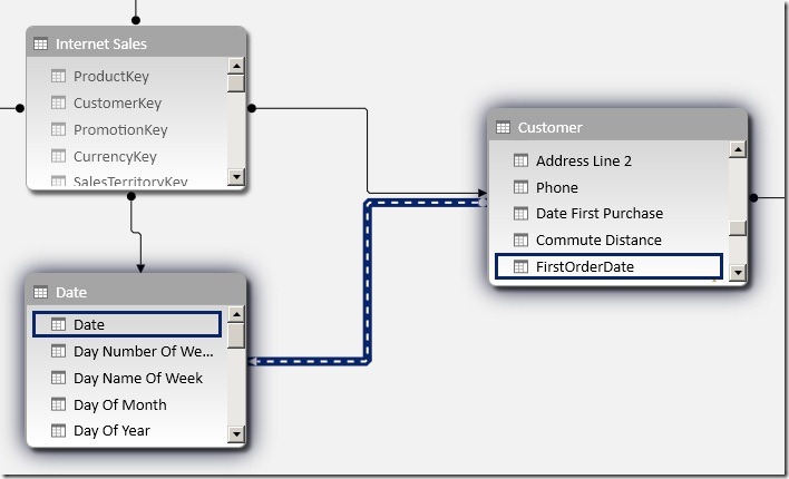
The above create calculated column allows us to relate our ‘Date’-table directly to our ‘Customer’-table. As there is already an existing relationship between those tables via ‘Internet Sales’ we have to create an inactive relationship at this point:

Customer_Date_Relationship

Using this new relationship we can very easy calculate customers that had their first sales in the selected period:

New Customers:=CALCULATE(
COUNTROWS(Customer),
USERELATIONSHIP(Customer[FirstOrderDate], ‘Date’[Date]))


Pretty neat, isn’t it?
We can use COUNTROWS() opposed to a distinct count measure as our ‘Customer’-table only contains unique customers – so we can count each row in the current filter context.
Another nice thing is that we do not have to use any Time-Intelligence function like DATESBETWEEN which are usually resolved using FILTER that would iterate over the whole table. Further it also works with all columns of our ‘Date’-table, no matter whether it is [Calendar Year], [Fiscal Semester] or [Day Name of Week]. (Have you ever wondered how many new customers you acquired on Tuesdays? 🙂 )   And finally, using USERELATIONSHIP allows us to use the full power of xVelocity as native relationships are resolved there.


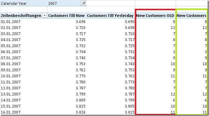
The results are of course the same as for [New Customers OLD]:

Result_Old_vs_New


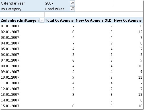
Though, there are still some issues with this calculation if there are filters on other tables:

Issue_Old_vs_New

As you can see, our new [New Customers] measure does not work in this situation as it is only related to our ‘Date’-table but not to ‘Product’.

I will address this issue in a follow-up post where I will also show how the final solution can be used for multidimensional models – Stay tuned!

Download Final Model (Office 2013!)


UPDATE: Part2 can be found here
Fiscal Periods, Tabular Models and Time-Intelligence

I recently had to build a tabular model for a financial application and I would like to share my findings on this topic in this post. Financial applications tend to have “Periods” instead of dates, months, etc. Though, those Periods are usually tied to months – e.g. January = “Period01”, February = “Period02” and so on. In addition to those “monthly periods” there are usually also further periods like “Period13”, “Period14” etc. to store manually booked values that are necessary for closing a fiscal year. To get the years closing value (for a P&L account) you have to add up all periods (Period01 to Period14). In DAX this is usually done by using TOTALYTD() or any similar Time-Intelligence Function.


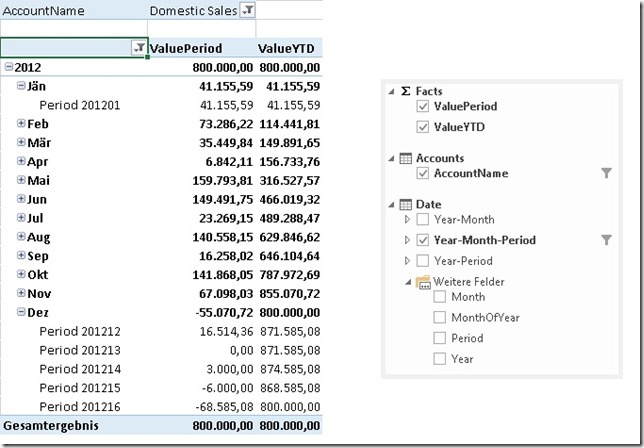
Here is what we want to achieve in the end. The final model should allow the End-user to create a report like this:

DesiredResult

This model allows us to analyze data by Year, by Month and of course also by Period. As you can see also the YTD is calculated correctly using DAX’s built-in Time-Intelligence functions.

However, to make use of Time-Intelligence functions a Date-table is required (more information: Time Intelligence Functions in DAX) but this will be covered later. Lets start off with a basic model without a Date-table.

For testing purposes I created this simple PowerPivot model:

BaseModel 

Sample of table ‘Facts’:

AccountID PeriodID Value
4 201201

41,155.59

2 201201

374,930.01

3 201211

525,545.15

5 201211

140,440.40

1 201212

16,514.36

5 201212

639,998.94

3 201213

-100,000.00

4 201213

20,000.00

5 201214

500,000.00


The first thing we need to do is to add a Date-table. This table should follow these rules:
– granularity=day –> one row for each date
– no gaps between the dates –> a contiguous range of dates
– do not use use the fact-table as your date-table –> always use an independent date-table
– the table must contain a column with the data type “Date” with unique values
– “Mark as Date-table”

A Date-table can be created using several approaches:
– Linked Table
– SQL view/table
– Azure Datamarket (e.g. Boyan Penev’s DateStream)
– …

(Creating an appropriate Date-table is not part of this post – for simplicity i used a Linked Table from my Excel workbook).

I further created calculated columns for Year, Month and MonthOfYear.


At this point we cannot link this table to our facts. We first have to create some kind of mapping between Periods and “real dates”. I decided to create a separate table for this purpose that links one Period to one Date. (Note: You may also put the whole logic into a calculated column of your fact-table.) This logic is straight forward for periods 1 to 11 which are simply mapped to the last (or first) date in that period. For Periods 12 and later this is a bit more tricky as we have to ensure that these periods are in the right order to be make our Time-Intelligence functions work correctly. So Period12 has to be before Period13, Period13 has to be before Period14, etc.

So I mapped Period16 (my sample has 16 Periods) to the 31st of December – the last date in the year as this is also the last period. Period 15 is mapped to the 30th of December – the second to last date. And so on, ending with Period12 mapped to the 27th of December:

PeriodID Date
201101 01/31/2011
201102 02/28/2011
201111 11/30/2011
201112 12/27/2011
201113 12/28/2011
201114 12/29/2011
201115 12/30/2011
201116 12/31/2011
201201 01/31/2012
201202 02/29/2012

I called the table ‘MapPeriodDate’.

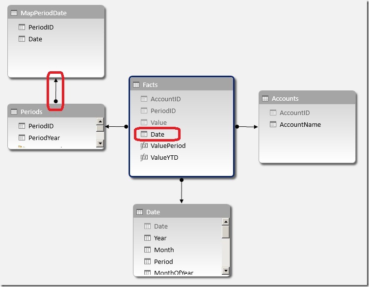
This table is then added to the model and linked to our already existing Period-table (Note: The table could also be linked to the Facts-table directly using PeriodID). This allows us to create a new calculated column in our Facts-table to get the mapping-date for the current Period:

=RELATED(MapPeriodDate[Date])


The new column can now be used to link our Facts-table to our Date-Table:

FinalModel

Please take care in which direction you create the relationship between ‘Periods’ and ‘MapPeriodDate’ as otherwise the RELATED()-function may not work!

Once the Facts-table and the Date-table are connected you may consider hiding the unnecessary tables ‘Periods’ and ‘MapPeriodDate’ as all queries should now use the Date-table. Also the Date-column should be hidden so the lowest level of our Date-table should be [Period].


To get a [Period]-column in our Date-table we have to create some more calculated columns:

[Period_LookUp]
= LOOKUPVALUE(MapPeriodDate[PeriodID], MapPeriodDate[Date], [Date])

this returns the PeriodID if the current date also exists in the MapPeriodDate-table. Note that we only get a value for the last date in a month.


[Period]
= CALCULATE(MIN([Period_LookUp]), DATESBETWEEN('Date'[Date], [Date], BLANK()))

our final [Period]-calculation returns the first populated value of [Period_LookUp] after the current date. The first populated value for dates in January is the 31st which has a value of 201101 – our PeriodID!


The last step is to create our YTD-measures. This is now very easy as we can again use the built-in Time-Intelligence functions with this new Date-table:

ValueYTD:=TOTALYTD(SUM([Value]), 'Date'[Date])

And of course also all other Time-Intelligence functions now work out of the box:

ValuePYTD:=CALCULATE([ValueYTD], DATEADD('Date'[Date], 1, YEAR))


All those calculations work with Years, Months and also Periods and offer the same flexibility that you are used to from the original financial application.


Download Final Model (Office 2013!)