Excel – Page 2 – Gerhard Brueckl on BI & Data

Fiscal Periods, Tabular Models and Time-Intelligence

Posted on 2013-02-12 by Gerhard Brueckl — 12 Comments ↓

I recently had to build a tabular model for a financial application and I would like to share my findings on this topic in this post. Financial applications tend to have “Periods” instead of dates, months, etc. Though, those Periods are usually tied to months – e.g. January = “Period01”, February = “Period02” and so on. In addition to those “monthly periods” there are usually also further periods like “Period13”, “Period14” etc. to store manually booked values that are necessary for closing a fiscal year. To get the years closing value (for a P&L account) you have to add up all periods (Period01 to Period14). In DAX this is usually done by using TOTALYTD() or any similar Time-Intelligence Function.

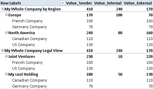
Here is what we want to achieve in the end. The final model should allow the End-user to create a report like this:

This model allows us to analyze data by Year, by Month and of course also by Period. As you can see also the YTD is calculated correctly using DAX’s built-in Time-Intelligence functions.

However, to make use of Time-Intelligence functions a Date-table is required (more information: Time Intelligence Functions in DAX) but this will be covered later. Lets start off with a basic model without a Date-table.

For testing purposes I created this simple PowerPivot model:

Sample of table ‘Facts’:

AccountID	PeriodID	Value
4	201201	41,155.59
2	201201	374,930.01
3	201211	525,545.15
5	201211	140,440.40
1	201212	16,514.36
5	201212	639,998.94
3	201213	-100,000.00
4	201213	20,000.00
5	201214	500,000.00

The first thing we need to do is to add a Date-table. This table should follow these rules:
– granularity=day –> one row for each date
– no gaps between the dates –> a contiguous range of dates
– do not use use the fact-table as your date-table –> always use an independent date-table
– the table must contain a column with the data type “Date” with unique values
– “Mark as Date-table”

A Date-table can be created using several approaches:
– Linked Table
– SQL view/table
– Azure Datamarket (e.g. Boyan Penev’s DateStream)
– …

(Creating an appropriate Date-table is not part of this post – for simplicity i used a Linked Table from my Excel workbook).

I further created calculated columns for Year, Month and MonthOfYear.

At this point we cannot link this table to our facts. We first have to create some kind of mapping between Periods and “real dates”. I decided to create a separate table for this purpose that links one Period to one Date. (Note: You may also put the whole logic into a calculated column of your fact-table.) This logic is straight forward for periods 1 to 11 which are simply mapped to the last (or first) date in that period. For Periods 12 and later this is a bit more tricky as we have to ensure that these periods are in the right order to be make our Time-Intelligence functions work correctly. So Period12 has to be before Period13, Period13 has to be before Period14, etc.

So I mapped Period16 (my sample has 16 Periods) to the 31st of December – the last date in the year as this is also the last period. Period 15 is mapped to the 30th of December – the second to last date. And so on, ending with Period12 mapped to the 27th of December:

PeriodID	Date
201101	01/31/2011
201102	02/28/2011
201111	11/30/2011
201112	12/27/2011
201113	12/28/2011
201114	12/29/2011
201115	12/30/2011
201116	12/31/2011
201201	01/31/2012
201202	02/29/2012

I called the table ‘MapPeriodDate’.

This table is then added to the model and linked to our already existing Period-table (Note: The table could also be linked to the Facts-table directly using PeriodID). This allows us to create a new calculated column in our Facts-table to get the mapping-date for the current Period:

=RELATED(MapPeriodDate[Date])

The new column can now be used to link our Facts-table to our Date-Table:

Please take care in which direction you create the relationship between ‘Periods’ and ‘MapPeriodDate’ as otherwise the RELATED()-function may not work!

Once the Facts-table and the Date-table are connected you may consider hiding the unnecessary tables ‘Periods’ and ‘MapPeriodDate’ as all queries should now use the Date-table. Also the Date-column should be hidden so the lowest level of our Date-table should be [Period].

To get a [Period]-column in our Date-table we have to create some more calculated columns:

[Period_LookUp] 
 = LOOKUPVALUE(MapPeriodDate[PeriodID], MapPeriodDate[Date], [Date])

this returns the PeriodID if the current date also exists in the MapPeriodDate-table. Note that we only get a value for the last date in a month.

[Period] 
 = CALCULATE(MIN([Period_LookUp]), DATESBETWEEN('Date'[Date], [Date], BLANK()))

our final [Period]-calculation returns the first populated value of [Period_LookUp] after the current date. The first populated value for dates in January is the 31st which has a value of 201101 – our PeriodID!

The last step is to create our YTD-measures. This is now very easy as we can again use the built-in Time-Intelligence functions with this new Date-table:

ValueYTD:=TOTALYTD(SUM([Value]), 'Date'[Date])

And of course also all other Time-Intelligence functions now work out of the box:

ValuePYTD:=CALCULATE([ValueYTD], DATEADD('Date'[Date], –1, YEAR))

All those calculations work with Years, Months and also Periods and offer the same flexibility that you are used to from the original financial application.

Download Final Model (Office 2013!)

FinancialPeriods.xlsx

Dynamic ABC Analysis in PowerPivot using DAX

Posted on 2013-01-28 by Gerhard Brueckl — 46 Comments ↓

An ABC Analysis is a very common requirement for for business users. It classifies e.g. Items, Products or Customers into groups based on their sales and how much impact they had on the cumulated overall sales. This is done in several steps.

I just published a new version of the Dynamic ABC Analysis at www.daxpatterns.com. The article can be found here.

1) Order products by their sales in descending order
2) Cumulate the sales beginning with the best selling product till the current product
3) Calculate the percentage of the cumulated sales vs. total sales
4) Assign a Class according to the cumulated percentage

Marco Russo already blogged about this here. He does the classification in a calculated column based on the overall sales of each product. As calculated columns are processed when the data is loaded, this is not dynamic in terms of your filters that you may apply in the final report. If, for example, a customer was within Class A regarding total sales but had no sales last year then a report for last year that uses this classification may give you misleading results.

In this blog I will show how to do this kind of calculation on-the-fly always in the context of the current filters. I am using Adventure Works DW 2008 R2 (download) as my sample data and create a dynamic ABC analysis of the products.

The first thing we notice is that our product table is a slowly changing dimension of type 2 and there are several entries for the same product as every change is traced in the same table.

So we want to do our classification on the ProductAlternateKey (=Business Key) column instead of our ProductKey (=Surrogate Key) column.

First we have to create a ranking of our products:

Rank CurrentProducts:=IF(HASONEVALUE(DimProduct[ProductAlternateKey]),

IF(NOT(ISBLANK([SUM SA])),

RANKX(

CALCULATETABLE(

VALUES(DimProduct[ProductAlternateKey]),

ALL(DimProduct[ProductAlternateKey])),

[SUM SA])))

Check if there is only one product in the current context and that this product also has sales. If this is the case we calculate our rank. We need to do the CALCULATETABLE to do the ranking within the currently applied filters on other columns of the DimProduct-table e.g. if a filter is applied to DimProduct[ProductSubcategoryKey] we want to see our ranking within that selected Subcategory and not against all Products.

I also created a measure [SUM SA] just to simplify the following expressions:

SUM SA:=SUM(FactInternetSales[SalesAmount])

The second step is to create a running total starting with the best-selling product/the product with the lowest rank:

CumSA CurrentProducts:=SUMX(

TOPN(

[Rank CurrentProducts],

CALCULATETABLE(

VALUES(DimProduct[ProductAlternateKey]),

ALL(DimProduct[ProductAlternateKey])),

[SUM SA]),

[SUM SA])

We use a combination of SUMX() and TOPN() here. TOPN() returns the top products ordered by [SUM SA]. Further we use our previously calculated rank to only get the products that have the same or more sales than the current product. For example if the current product has rank 3 we sum up the top 3 products to get our cumulated sum (=sum of the first 3 products) for this product. Again we need to use CALCULATETABLE() to retain other filters on the DimProduct-table.

The third step is pretty easy – we need to calculate percentage of the cumulated sales vs. the total sales:

CumSA% CurrentProducts:=

[CumSA CurrentProducts]

/

CALCULATE([SUM SA], ALL(DimProduct[ProductAlternateKey]))

This calculation is straight forward and should not need any further explanation.

The result of those calculations can be seen here:

To do our final classification we have to extend our model with a new table that holds our classes and their border-values:

Class	LowerBoundary	UpperBoundary
A	0	0.7
B	0.7	0.9
C	0.9	1

Class A should contain products which’s cumulated sales are between 0 and 0.7 – between 0% and 70%.
Class B should contain products which’s cumulated sales are between 0.7 and 0.9 – between 70% and 90%.
etc.

(This table can later be extended to support any number of classes and any boundaries between 0% and 100%.)

To get the boundaries of the selected class we create two measures that are later used in our final calculation:

MinLowerBoundary:=MIN([LowerBoundary])

MaxUpperBoundary:=MAX([UpperBoundary])

Our final calculation looks like this:

SA Classified Current:=IF(NOT(ISCROSSFILTERED(Classification[Class])),

[SUM SA],

CALCULATE(

[SUM SA],

FILTER(

VALUES(DimProduct[ProductAlternateKey]),

[MinLowerBoundary] < [CumSA% CurrentProducts]

&& [CumSA% CurrentProducts] <= [MaxUpperBoundary])))

If our Classification-table is not filtered, we just show our [SUM SA]-measure. Otherwise we extend the filter on our DimProduct[ProductAlternateKey] using our classification filtering out all products that do not fall within the borders of the currently selected class.

This measure allows us to see the changes of the classification of a specific product e.g. over time:

In 2006 our selected product was in Class C. For 2007 and 2008 it improved and is now in Class A. Still, overall it resides in Class B.

We may also analyze the impact of our promotions on the sales of our classified products:

Our Promotion “Touring-1000 Promotion” only had impact on products in Class C so we may consider to stop that promotion and invest more into the other promotions that affect all classes.

The classification can be used everywhere you need it – in the filter, on rows or on columns, even slicers work. The only drawback is that the on-the-fly calculation can take quite some time. If I find some time in the future i may try to further tune them and update this blog-post.

The example workbook can be downloaded here:

Dynamic ABC Analysis.xlsx

Though it is already in Office 2013 format an may not be opened with any previous versions of Excel/PowerPivot.
It also includes a second set of calculations that use the same logic as described above but does all the calculations without retaining any filters on the DimProducts-table. This allows you to filter on Class “A” and ProductSubcategory “Bike Racks” realizing that “Bike Racks” are not a Class “A” product or to see which Subcategories or Categories actually contain Class A, B or C products!

Consolidation and Intercompany Elimination with parallel hierarchies

Posted on 2012-05-31 by Gerhard Brueckl — 2 Comments ↓

In my last post I described and approach on how to calculate consolidated values (adjusted by intercompany eliminations) using PowerPivot and DAX. In this post I will extend this technique so it can also be used with parallel hierarchies as this is also very common in financial applications.

Switching from a single hierarchy to multiple parallel hierarchies has several drawbacks for tabular models:
1) business keys cannot be used to build the PC-hierarchy as they are not unique anymore
2) artificial keys and parent-keys are required
3) as business keys are not unique anymore, we also cannot create a relationship between facts and our dimension
4) PowerPivot tables do not support “UNION” to load several single hierarchies and combine them

All the issues described above have to be handled before the hierarchies can be loaded into PowerPivot. This is usually done in a relational database but this will not be covered in this post.

For simplicity I created a table in Excel that already has the correct format:

ID	ParentID	SenderID	Name
1		TOT	My Whole Company by Region
2	1	EUROPE	Europe
3	2	GER	Germany Company
4	2	FR	French Company
5	1	NA	North America
6	5	USA	US Company
7	5	CAN	Canadian Company
-99		EXTERNAL	EXTERNAL
8		TOT_2	My Whole Company Legal View
9	8	JV	Joint Ventures
10	9	FR	French Company
11	9	USA	US Company
12	8	HOLD	My cool Holding
13	12	GER	Germany Company
14	12	CAN	Canadian Company

We have 2 parallel hierarchies – “My Whole Company by Region” and “My Whole Company Legal View”. In PowerPivot this looks like this:

Each Company can be assigned to different nodes in every hierarchy.

As I already noted above, the SenderIDs are not unique anymore, and therefore we cannot create a relationship to our fact-table. So we have to handle this in our calculation. The approach is similar to handling SCD2 dimensions in PowerPivot what I described in previous posts (Part1 and Part2). We use CONTAINS-function to filter our fact-table based on the currently active SenderIDs in the dimension-table:

Value_Sender:=
CALCULATE([Value_SUM],
FILTER(
     'Facts',
     CONTAINS(
          'Sender',
          'Sender'[SenderID],
          'Facts'[SenderID]))
)

Actually this is the only difference in the calculation when we are dealing with multiple parallel hierarches. The other calculations are the same with the only difference that we have to use [Value_Sender] instead of [Value_SUM]:

Value_Internal:=
 CALCULATE([Value_Sender],
 FILTER(
      'Facts',
      CONTAINS(
           'Sender',
           'Sender'[SenderID],
           'Facts'[ReceiverID]))
 )

and

Value_External:=
 CALCULATE([Value_Sender],
 FILTER(
      'Facts',
      NOT(
           CONTAINS(
                'Sender',
                'Sender'[SenderID],
                'Facts'[ReceiverID])))
 )

As you can see this approach also works very well with multiple hierarchies. In the end we get the desired results:

Taking a look at “My cool Holding” we see that a value of 50 is eliminated as there have been sales from CAN to GER. On top-level of the hierarchy we see the same values being eliminated (170) as both hierarchies contain the same companies and therefore only sales to EXTERNAL can summed up to get the correct value.

As this technique operates on leaf-level it works with all possible hierarchies regardless of how many companies are assigned to which node or how deep the hierarchies are!

(Just to compare the values from above – the fact-table is the same as in the previous post: )

SenderID	ReceiverID	Value
FR	GER	100
CAN	GER	50
GER	EXTERNAL	70
USA	CAN	30
USA	FR	10
USA	EXTERNAL	90
CAN	USA	50
CAN	EXTERNAL	10

ISO 8601 Week in DAX

Posted on 2012-04-20 by Gerhard Brueckl — 23 Comments ↓

I recently built a PowerPiovt model where I had to display weeks according to ISO 8601. As I came across this frequently in the past when I developed SQL Server databases (prior to 2008) I was aware that ISO weeks can also be calculated using some complex logics. When I discussed this with some of my colleagues during a training, one of the attendees told me, that this can be solved in Excel very easily using Excels WEEKNUM()-function. This function takes to arguments:

Serial_num is a date within the week. Dates should be entered by using the DATE function, or as results of other formulas or functions. For example, use DATE(2008,5,23) for the 23rd day of May, 2008. Problems can occur if dates are entered as text.

Return_type is a number that determines on which day the week begins. The default is 1.

Return_type	Week Begins
1	Week begins on Sunday. Weekdays are numbered 1 through 7.
2	Week begins on Monday. Weekdays are numbered 1 through 7.

According to Excels Online-Help the second parameter only supports values 1 and 2. But this is not 100% true. You can also use the value 21 as second parameter, and guess what – it now returns weeknumbers according to ISO 8601. As many DAX-functions are derived from Excel (including WEEKNUM()-function), this also works with DAX’s WEEKNUM()-function!

So by creating a calculated column as

=WEEKNUM([Date], 21)

you get the ISO week number for the current [Date].

If you also want to calculate “ISO years” to build clean hierarchies you may want to use this formula in an other calculated column:

=IF([ISOWeek]<5 && [CalendarWeek] > 50;
     [Year]+1;
     IF([ISOWeek]>50 && [CalendarWeek]<5; 
          [Year]-1; 
          [Year]))

I think we can learn a lot from experienced Excel-users here as most tricks also work in PowerPivot/DAX!

If you want to do the same in Power Query already, here is some sample code (original source)

let
    StartDate        = #date (2009,1,1),
    EndDate          = #date (2024,12,31),
    ListOfDates      = List.Dates(StartDate, DurationDays, #duration(1, 0, 0, 0)),
    DurationDays     = Duration.Days (EndDate - StartDate) + 1,
    TableOfDates     = Table.FromList(ListOfDates, Splitter.SplitByNothing(), null, null, ExtraValues.Error),
    DateColText      = Table.RenameColumns(TableOfDates,{{"Column1", "Date"}}),
    DateCol          = Table.TransformColumnTypes(DateColText,{{"Date", type date}}),
    WeekdayCol       = Table.AddColumn(DateCol, "Weekday Number", each Date.DayOfWeek([Date], Day.Monday) + 1,Int64.Type),
    IsoWeekYearCol   = Table.AddColumn(WeekdayCol, "Iso Week Year", each Date.Year(Date.AddDays([Date], 4-[Weekday Number])), Int64.Type),
    IsoWeekNrCol     = Table.AddColumn(IsoWeekYearCol, "Iso Week Nummer", each (Duration.Days(Date.AddDays([Date], 4-[Weekday Number]) - #date([Iso Week Year], 1 , 7 - Date.DayOfWeek(#date([Iso Week Year],1,4), Day.Monday)))/7)+1, Int64.Type),
    IsoWeekdayExtCol = Table.AddColumn(IsoWeekNrCol, "Iso Weekday Extended", each Text.From([Iso Week Year]) & "-W" & Text.End("0" &     Text.From([Iso Week Nummer]), 2) & "-"&  Text.From([Weekday Number]))
in
    IsoWeekdayExtCol

Synchronizing PivotTable Filters without using VBA

Posted on 2012-04-03 by Gerhard Brueckl — 6 Comments ↓

I recently did a workshop with one of my customers where we were building a PowerPivot model which was later used for several reports. The final workbook contained 10+ worksheets each with one or more PivotTables querying the PowerPivot model. Most of the PivotTables had several filters in common. For example Year, Period, Organisation and so on. A very important requirement for the customer was that whenever one of those filters is changed, all other PivotTables in the workbook should also be synchronized and filtered accordingly.

A common solution for this problem is to use a VBA-Macro that pushes changes in the filter across all PivotTables. This approach is described in many blogs and/or forum entries:
http://www.excelforum.com/excel-programming/778048-synchronizing-two-pivot-tables-of-same-data-with-one-report-filter.html
http://www.ozgrid.com/forum/showthread.php?t=87519

This solutions works fine but has the same drawback as all other VBA Macros:

Users may need special security to use macros as they could be unsafe
Macros may be forbidden by your company
and (especially for BI) THEY DO NOT WORK WITH EXCEL SERVICES!!!

Also for my customer macros have not been an option. As I could not find any other solution in the web, I was very happy when one of my colleagues showed me an other option to solve this issue.
We did not use any macros but only used native, built-in excel functionalities – Slicers.

And this is how it works:

Create a two PivotTables on top of your datasource (I tested multidimensional and tabular datasources, but I assume that this will also work for all other datasources)
Add the same field(s) to the Report-Filter of your PivotTables
Use rows, columns and values as you like

In my example I used the Adventore Works cube and created the following worksheet:

I used [Date].[CalendarYear] in both PivotTables as a filter. As you already know these filters are independent of each other usually.

To solve the initial problem and keep them in sync you first have to add a new slicer also for [Date].[CalendarYear]

and connect it to both PivotTables:

And that’s actually all you have to do!

Now you can either change the filter of PivotTable1, PivotTable2 or use the slicer to select your CalendarYear. The selection will be propagated through all objects that are connected to the slicer!

Another neat feature of slicers is, that the do not have to reside on the same worksheet as the connected PivotTables. So you could also move them to a hidden worksheet and everything will still work!

Also multiselects work just fine!

You may also want to put hierarchies into the filter – this also works
But be aware that one slicer is created for each hierarchy-level!

I have not tested this solution in Excel-Services and SharePoint yet but I assume that it will also work there. When I have some more time I will test this and post my results.

UPDATE: I just ran some tests on SharePoint and this solution also works with Excel-Services

Share this:

I just published a new version of the Dynamic ABC Analysis at www.daxpatterns.com. The article can be found here.

Share this:

Share this:

Share this:

Share this: