Dynamic ABC Analysis in Power Pivot using DAX – Part 2

Almost two years ago I published the first version of an Dynamic ABC Analysis in Power Pivot and by now it is the post with the most comments among all my blog posts. This has two reason:
1) the formula was quite complex and not easy to understand or implement
2) the performance was not really great with bigger datasets

When the first of those comments flew in, I started investigating into a new, advanced formula. At about the same time Marco Russo and Alberto Ferrari published their ABC Classification pattern – a static version using calculated columns – at www.daxpatterns.com. When I had my first dynamic version ready I sent it to Marco and Alberto and asked if they are interested in the pattern and if I can publish it on their website. Long story short – this week the new pattern was released and can now be found here:

ABC Classification – Dynamic

It got some major performance improvements and was also designed towards reusability with other models. The article also contains some detailed explanations how the formula actually works but its still very hard DAX which will take some time to be fully understood. The pattern also features some extended versions to address more specific requirements but I think its best to just read the article on your own.

Hope you enjoy it!

Events-In-Progress for Time Periods in DAX

Calculating the Events-In-Progress is a very common requirement and many of my fellow bloggers like Chris Webb, Alberto Ferrari and Jason Thomas already blogged about it and came up with some really nice solutions. Alberto also wrote a white-paper summing up all their findings which is a must-read for every DAX and Tabular/PowerPivot developer.
However, I recently had a slightly different requirement where I needed to calculate the Events-In-Progress for Time Periods – e.g. the Open Orders in a given month – and not only for a single day. The calculations shown in the white-paper only work for a single day so I had to come up with my own calculation to deal with this particular problem.

Before we can start we need to identify which orders we actually want to count if a Time Period is selected. Basically we have to differentiate between 6 types of Orders for our calculation and which of them we want to filter or not:
Overview_EventsInProgress_TimeFrame

Order Definition
Order1 (O1) Starts before the Time Period and ends after it
Order2 (O2) Starts before the Time Period and ends in it
Order3 (O3) Starts in the Time Period and ends after it
Order4 (O4) Starts and ends in the Time Period
Order5 (O5) Starts and ends after the Time Period
Order6 (O6) Starts and ends before the Time Period

For my customer an order was considered as “open” if it was open within the selected Time Period, so in our case we need to count only Orders O1, O2, O3 and O4. The first calculation you would usually come up with may look like this:

  1. [MyOpenOrders_FILTER] :=
  2. CALCULATE (
  3.     DISTINCTCOUNT ( ‘Internet Sales’[Sales Order Number] ),
  4.     FILTER (
  5.         ‘Internet Sales’,
  6.         ‘Internet Sales’[Order Date]
  7.             <= CALCULATE ( MAX ( ‘Date’[Date] ) )
  8.     ),
  9.     FILTER (
  10.         ‘Internet Sales’,
  11.         ‘Internet Sales’[Ship Date]
  12.             >= CALCULATE ( MIN ( ‘Date’[Date] ) )
  13.     )
  14. )
[MyOpenOrders_FILTER] :=
CALCULATE (
    DISTINCTCOUNT ( 'Internet Sales'[Sales Order Number] ), -- our calculation, could also be a reference to measure
    FILTER (
        ‘Internet Sales’,
        ‘Internet Sales’[Order Date]
            <= CALCULATE ( MAX ( 'Date'[Date] ) )
    ),
    FILTER (
        ‘Internet Sales’,
        ‘Internet Sales’[Ship Date]
            >= CALCULATE ( MIN ( 'Date'[Date] ) )
    )
)

We apply custom filters here to get all orders that were ordered on or before the last day and were also shipped on or after the first day of the selected Time Period. This is pretty straight forward and works just fine from a business point of view. However, performance could be much better as you probably already guessed if you read Alberto’s white-paper.

So I integrate his logic into my calculation and came up with this formula (Note that I could not use the final Yoda-Solution as I am using a DISTINCTCOUNT here):

  1. [MyOpenOrders_TimePeriod] :=
  2. CALCULATE (
  3.     DISTINCTCOUNT ( ‘Internet Sales’[Sales Order Number] ),
  4.     GENERATE (
  5.         VALUES ( ‘Date’[Date] ),
  6.         FILTER (
  7.             ‘Internet Sales’,
  8.             CONTAINS (
  9.                 DATESBETWEEN (
  10.                     ‘Date’[Date],
  11.                     ‘Internet Sales’[Order Date],
  12.                     ‘Internet Sales’[Ship Date]
  13.                 ),
  14.                 [Date], ‘Date’[Date]
  15.             )
  16.         )
  17.     )
  18. )

To better understand the calculation you may want to rephrase the original requirement to this: “An open order is an order that was open on at least one day in the selected Time Period”.

I am not going to explain the calculations in detail again as the approach was already very well explained by Alberto and the concepts are the very same.

An alternative calculation would also be this one which of course produces the same results but performs “different”:

  1. [MyOpenOrders_TimePeriod2] :=
  2. CALCULATE (
  3.     DISTINCTCOUNT ( ‘Internet Sales’[Sales Order Number] ),
  4.     FILTER (
  5.         GENERATE (
  6.             SUMMARIZE (
  7.                 ‘Internet Sales’,
  8.                 ‘Internet Sales’[Order Date],
  9.                 ‘Internet Sales’[Ship Date]
  10.             ),
  11.             DATESBETWEEN (
  12.                 ‘Date’[Date],
  13.                 ‘Internet Sales’[Order Date],
  14.                 ‘Internet Sales’[Ship Date]
  15.             )
  16.         ),
  17.         CONTAINS ( VALUES ( ‘Date’[Date] ), [Date], ‘Date’[Date] )
  18.     )
  19. )

I said it performs “different” as for all DAX calculations, performance also depends on your model, the data and the distribution and granularity of the data. So you should test which calculation performs best in your scenario. I did a simple comparison in terms of query performance for AdventureWorks and also my customer’s model and results are slightly different:

Calculation (Results in ms)   AdventureWorks   Customer’s Model
[MyOpenOrders_FILTER]                   58.0              1,094.0
[MyOpenOrders_TimePeriod]                   40.0                  390.8
[MyOpenOrders_TimePeriod2]                   35.5                  448.3

As you can see, the original FILTER-calculation performs worst on both models. The last calculation performs better on the small AdventureWorks-Model whereas on my customer’s model (16 Mio rows) the calculation in the middle performs best. So it’s up to you (and your model) which calculation you should prefer.

The neat thing is that all three calculations can be used with any existing hierarchy or column in your Date-table and of course also on the Date-Level as the original calculation.

Download: Events-in-Progress.pbix

Using Self-Signed Certificates for your Power BI DMG

In my previous post I showed how to setup a Power BI Data Management Gateway on a non-domain Azure VM. The final setup is also the starting-point for this post where we will use self-signed certificates to use HTTPS/SSL connectivity to our DMG. So make sure that you have all prerequisites up and running before you continue reading.

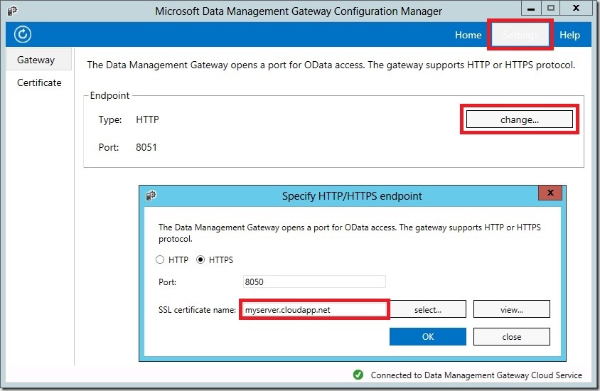
Basically, the process to switch to HTTPS is pretty straight forward. Simply open your DMG, go to Settings and change from HTTP to HTTPS. Finally select your certificate and you are ready to go!
This may work in a corporate hybrid environment where everything is set up correctly but for a non-Azure VM this is a bit more complicated and this is what this post is about.

Besides the initial setup from my previous post there are some steps you need to do in advance in order for HTTPS connectivity to work:
1) Open the port that the DMG HTTPS connection uses in your Windows Firewall (default is port 8050)
2) Create an Endpoint for your Azure VM for the very same port
3) Create a self-signed certificate to be used to establish a secure connection

You should already be familiar with 1) and 2) as you needed to do the same steps also for your HTTP port of your DMG (default is port 8051 here). To create a self-signed certificate you can simply follow the steps as described here. The important thing here is to use the full qualified server name: CN=myserver.cloudapp.net
This is very import, otherwise the final connection will not work!

Your MakeCert-command should look similar to this:
makecert -r -pe -n “CN=myserver.cloudapp.net” -b 01/01/2000 -e 01/01/2050 -eku 1.3.6.1.5.5.7.3.1 -ss my -sr localMachine -sky exchange -sp “Microsoft RSA SChannel Cryptographic Provider” -sy 12

After you run the command the new certificate is automatically added to your users personal certificates and can be used when setting up HTTPS connectivity for your DMG:
SetupDMG

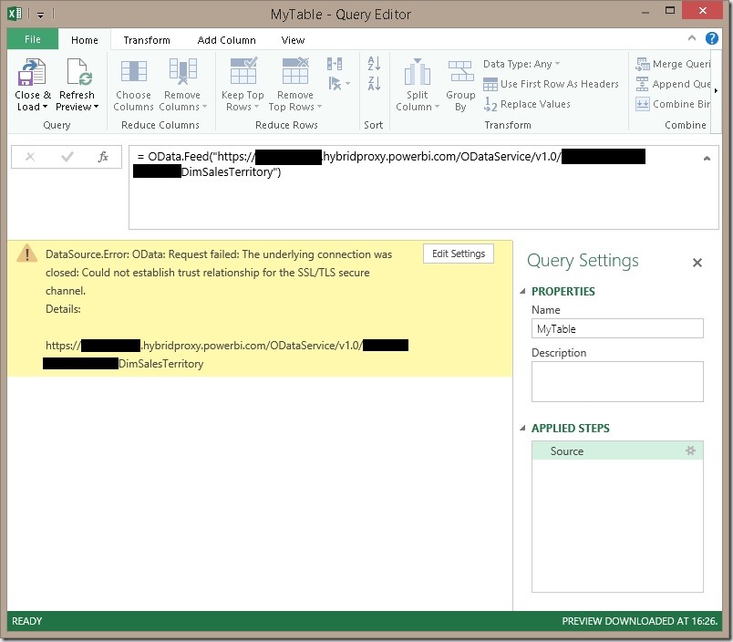
Once you click [OK] it takes some time (~1 Minute) until everything is updated and HTTPS connectivity can be used. Now you can use Excel and Power Query to search for your data sources that are published via OData. You will find all of them but as soon as you try to load the data you will receive the following error:
ErrorPQ

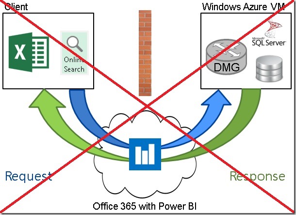
That’s a bit surprising as the DMG is configured correctly using HTTPS and the very same OData feed worked just fine with HTTP. But here comes the error in my thinking that I was not aware of before talking to Benjamin Tang and Samuel Zhang from the product team. Until that point I always thought that the data is load through the cloud and there is no direct connection from my client to the server:
WrongConnectivityThought
But this is not how it works!

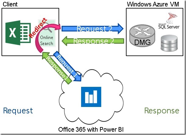
What actually happens in the background is that the request to the Power BI OData service gets redirected to the server and the client connects directly to the server:
ActualConnection

And this is also where our PQ error originates as the certificate used is not a trusted certificate on the client. In order to make it a trusted certificate you need to install it on the client. This can be done by following these steps:
1) Launch Internet Explorer using “Run as Administrator”
    (I’m serious here, this only works with IE but not with e.g. Chrome!)
2) navigate to https://myserver.cloudapp.net:8050 (or whatever servername/port you used)
3) continue to the website and ignore the certificate error
4) press [Cancel] at the popup the asks for credentials
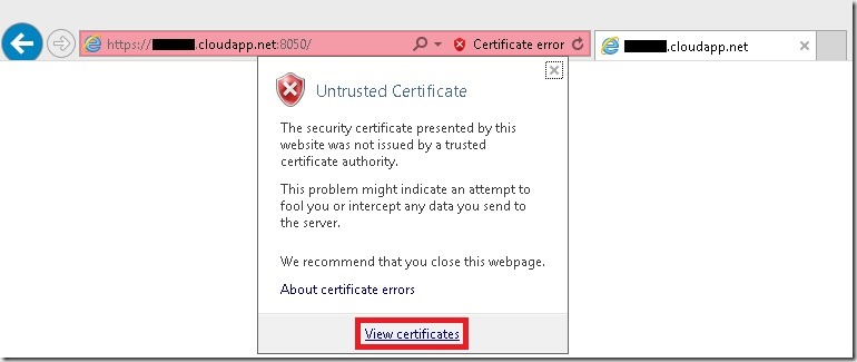
5) now click on the “Certificate error” in the menu bar and press “View certificates”
ViewCertificate
6) Now install the certificate:
InstallCertificate
(Please note that this option is only available if you are using Internet Explorer launched as Administrator!!!)
7) select the location where you want to store the certificate (Current User or Local Machine depending whether it should be installed for you only or for all users)
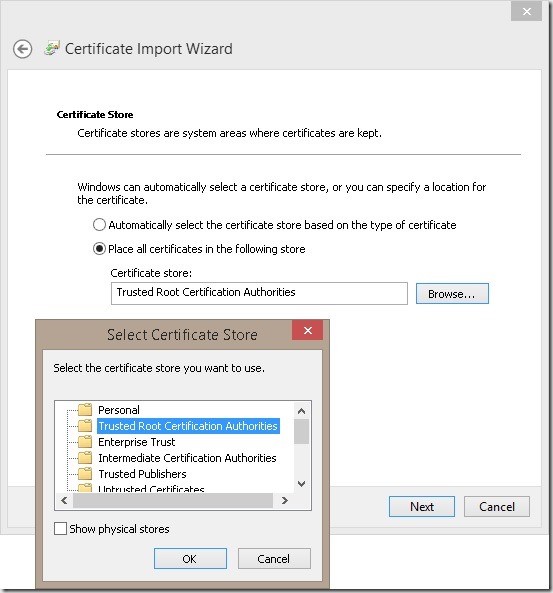
8) whichever storage location you used, just make sure that you place the certificate in the “Trusted Root Certification Authorities” on the next page:
InstallCertificateStore

Once you have installed the certificate to your Trusted Root Certificate Authorities store the Power Query connections works again but now it is using HTTPS!

Of course this solution is only for demo and testing purposes, in a real world scenario you would already have your certificates in place and everything should indeed work out-of-the-box.

Using Power BI DMG on Non-Domain Azure VMs – August 2014 Update

In one of my recent posts I explained how to use the Power BI Data Management Gateway to access data hosted in a SQL Server running on an Azure VM. At the time of writing that post the steps to establish connectivity were not quite intuitive. With the latest Update of the Data Management Gateway (Version 1.2.5303.1 and later) things got a bit easier. However, there is still a little thing that you have to configure to make everything work smoothly. First of all, I highly recommend you to read my first post on this topic to fully understand the actual issue and why it does not work out-of-the-box.

When creating a new Data Source the DMG has to be reachable from the machine on which the Data Source Manager (the Click-Once application where you enter your SQL credentials) is executed. The hostname is derived from the DMG and for Azure VMs this does by default not reflect the hostname under which the VM is reachable from public. The hostname would be “MyServer” whereas the public DNS name is “MyServer.cloudapp.net”. To check what hostname the DMG is using you can execute the following Power Shell command:

  1. [System.Net.Dns]::GetHostEntry("localhost")

In order to change this hostname you can either join the VM to a domain (which is not what we want to do here) or use the following approach:

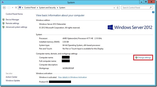
Open the System settings of your server:
SystemSettings_default
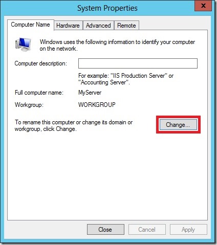
You will notice that both, “Computer name” and “Full computer name” show the same name, and both without the suffix “.cloudapp.net”. In order to change this we need to click the “Change settings” button right next to the names to open the System Properties:
SystemProperties

Again, click [Change …] to open the computers domain settings:
DomainSettings
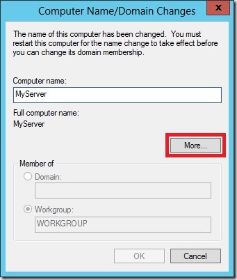
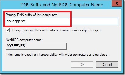
As you can see, the “Full computer name” does not show our required suffix “.cloudapp.net” yet. We can change this in the dialog available via the [More …] Button:
DNS_Settings
Here we can set our “Primary DNS suffix” – we set it to “cloudapp.net” (without leading dot) to reflect our public DNS name.

By clicking [OK] on all open windows you will see the new full name “MyServer.cloudapp.net” now being used as “Full computer name” everywhere. Also our Power Shell command from above now shows the correct hostname. Note that this change also requires a reboot of the VM.

Once the machine is rebooted and DMG is running again you can now use any client machine to create your Data Source which was previously only possible from the server directly and required a RDP connection. Also HTTPS connectivity with self-signed certificates works with this approach which I will show in one of my next posts – so stay tuned!

Restoring a SSAS Tabular Model to Power Pivot

It is a very common scenario to create a SSAS Tabular Model out of an Power Pivot Model contained in an Excel workbook. Microsoft even created an wizard (or actually a separate Visual Studio project) that supports you doing this. Even further, this process is also a major part of Microsoft’s strategy to cover Personal BI, Team BI and Corporate BI within one technology being xVelocity. This all works just fine but there may also be scenarios where you need to do it the other way round – converting a Tabular model to Power Pivot. Several use-cases come into my mind but I am sure that the most important one is to making data available offline for e.g. sales people to take it with them on their every day work. And in this blog post I will show how this can be done!

But before taking a closer look into how this can be accomplished, lets first see how the import from Power Pivot to SSAS Tabular works. To do this start SQL Server Profiler and connect to your tabular instance. Then create a new Tabular project in Visual Studio based on an existing Power Pivot workbook. At this point you will notice a lot of events happening on our SSAS Tabular server. The most important event for us is “Command End” with the EventSubclass “9 – restore”:
RestoreFromPowerPivot

SSAS actually restores a backup from a “Model.abf” backup file which is located in our project directory that we just created:
BackupExtractedFromPowerPivot

So far so good – but where does this file come from?

Well, the origin of the file has to be our Excel workbook that we imported. Knowing that all new office formats ending with “x” (.xlsx, .docx, …) are basically ZIP files, we can inspect our original Excel workbook by simply rename it to “.zip”. This allows us to browse the Excel file structure:
ExcelUnzipped

We will find a folder called “xl” which contains a sub-folder called “model”. This folder contains one item called “item.data”. If you take a closer look at the file size you may realize that both, the “Model.abf” file that we restored and the “item.data” file from our Excel workbook have the exact same size:
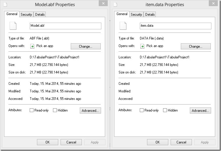
FileProperties

A Coincidence? Not really!

What happens behind the scenes when you import a Power Pivot model into SSAS Tabular is that this “item.data” file gets copied into your project directory and is renamed to “Model.abf” and then restored to the SSAS Tabular workspace instance by using an standard database restore.

Having this information probably makes you think: If it works in one direction, why wouldn’t it also work the other way round? And it does!

So here are the steps that you need to do in order to restore your SSAS Tabular backup into an Excel Power Pivot workbook:

  1. Create a backup of your SSAS Tabular database and rename it to “item.data”
  2. Create an empty Excel workbook and add a simple linked table to the Excel data model (which is actually Power Pivot).
    This is necessary to tell Excel that the workbook contains a Power Pivot model which has to be loaded once the file is opened.
  3. Close the Excel workbook and rename it from “MyFile.xlsx” to “MyFile.xlsx.zip”
  4. Open the .zip-file in Windows Explorer and locate the “\xl\model\”-folder
  5. Replace the “item.data” file with the file that you created in step 1.
  6. Rename the .zip-file back to “MyFile.xlsx”
  7. Open the Excel Workbook
  8. Voilá! You can now work with the data model as with any other Power Pivot model!

I tested this with a SSAS Tabular backup from SQL Server 2012 SP1 being restored to the streamed version of Excel from Office 365 with the latest version of Power Pivot. I assume that it also works with older versions but have not tested all combinations yet.

There are also some features that will not work, for example roles. If your Tabular database contains roles you will not be able to use this approach. Excel will complain that the Power Pivot model is broken. However, other Tabular features like partitions actually work with the little limitation that you cannot change them later on in the Power Pivot model or process them separately:
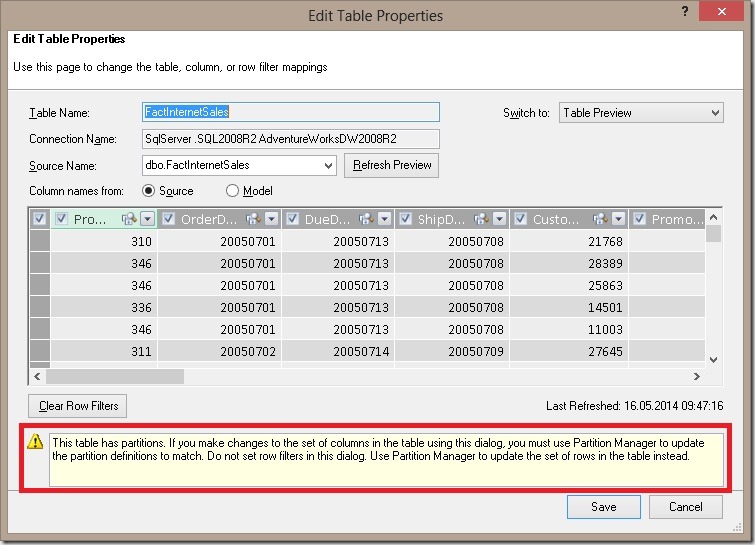
PowerPivotPartitions
Another thing to note here is that only up to 3 partitions are allowed, otherwise you will get the same error as for roles. I think this is related to the limitation of 3 partitions for SQL Server Analysis Services Standard Edition as Chris Webb described here.

Besides these obvious features there are also some other cool things that you can do in Tabular which are not possible in Power Pivot. Most (or actually all) of them are accessible only by using BIDS Helper – a great THANK YOU to the developers of BIDS Helper at this point!
BIDS Helper enables you to add classical multidimensional features also to Tabular models which is not possible using standard Visual Studio only. Those include:

  • DisplayFolders
  • Translations (metadata only)
  • Actions

I tested it for DisplayFolders and Actions and both are working also in Power Pivot after the backup was restored and I further assume that all the other things will also work just fine.
Simply keep in mind that Power Pivot is basically a fully featured Analysis Services instance running within Excel!

For my (and your) convenience I also created a little PowerShell script that does all the work:

  1. # Load the assembly with the ZipFile class
  2. [System.Reflection.Assembly]::LoadWithPartialName("System.IO.Compression.FileSystem") | Out-Null
  3. # Load the assembly to access Analysis Services
  4. [System.Reflection.Assembly]::LoadWithPartialName("Microsoft.AnalysisServices") | Out-Null
  5. # Also install "Analysis Services PowerShell" according to http://technet.microsoft.com/en-us/library/hh213141.aspx
  6.  
  7. # INPUT-Variables, change these to match your environment
  8. $rootFolder = "D:\Test_PowerShell\"
  9. $emptyExcelFile = $rootFolder + "EmptyExcel.xlsx"
  10. $ssasServerName = "localhost\TAB2012"
  11. $ssasDatabaseName = "AdventureWorks"
  12.  
  13. # internal variables
  14. $newExcelFile = $rootFolder + $ssasDatabaseName + ".xlsx"
  15. $newExcelFileZip = $newExcelFile + ".zip"
  16. $unzipFolder = $rootFolder + "TEMP_ExcelUnzipped"
  17. $backupFile = $rootFolder + $ssasDatabaseName + ".abf"
  18. $itemDestination = $unzipFolder + "\xl\model\item.data"
  19.  
  20. # Copy the empty Excel file and rename it to ".zip"
  21. Copy-Item -Path $emptyExcelFile -Destination $newExcelFileZip
  22.  
  23. # Unzip the file using the ZipFile class
  24. [System.IO.Compression.ZipFile]::ExtractToDirectory($newExcelFileZip, $unzipFolder)
  25.  
  26. # Create a backup of the SSAS Tabular database
  27. Backup-ASDatabase -Server $ssasServerName -Name $ssasDatabaseName -BackupFile $backupFile -AllowOverwrite -ApplyCompression
  28.  
  29. # Copy the backup-file to our extracted Excel folder structure
  30. Copy-Item -Path $backupFile -Destination $itemDestination -Force
  31.  
  32. # Check if the target file exists and delete it
  33. if (Test-Path -Path $newExcelFile) { Remove-Item -Path $newExcelFile }
  34.  
  35. # Zip the folder-structure again using the ZipFile class and rename it to ".xlsx"
  36. [System.IO.Compression.ZipFile]::CreateFromDirectory($unzipFolder, $newExcelFile)
  37.  
  38. # Cleanup the unecessary files
  39. Remove-Item -Path $unzipFolder -Recurse
  40. Remove-Item -Path $backupFile
  41. Remove-Item -Path $newExcelFileZip

The last thing to mention here is that I don’t know if this is officially supported in any way by Microsoft – actually I am pretty sure it is not – so watch out what you are doing and don’t complain if something is not working as expected.

Using Power BI Data Management Gateway on Non-Domain Azure VM

UPDATE AUGUST 2014:
There were some changes to the DMG in August 2014. Please refer to my new blog post which addresses the issues with the new version! However, I still recommend you to read this post first in order to fully understand the original issue!
The new post can be found here.


I am currently preparing some demos and examples for Power BI. As you can expect for demos you do not want to put too much effort in building up any infrastructure so I decided to use an Azure VM to host my SQL databases and SSAS cubes. Keeping things simple the Azure VM is not joined to a domain which is fine for SQL where I can use SQL authentication, for SSAS I use msmdpump.dll. After everything was set up I wanted to install the Data Management Gateway to expose my SQL tables via OData to Power Query and Online Search.
Bryan C. Smith recently published an article on that very same topic Creating a Demo Power BI Data Gateway using an Azure Virtual Machine but for some reasons it did not work for me. Further, as Bryan already mentions in the first paragraph, his setup is not supported and  its also a bit of a hack (modifying hosts-file, and so on).
So I started my own investigations and came up with another solution, which only uses out-of-the-box features and tools and is actually quite simple. Another thing to mention here is that it will (probably) not work for scheduled data refreshes but only for exposing the SQL database via OData and make it searchable in Power Query.
Having that said, here are the steps to follow:

1) Setup the Data Management Gateway itself on the Azure VM as described here: Create a Data Management Gateway. This should work just fine and the Gateway should be in the “Registered”-state on the Azure VM and in “Ready”-state in the Power BI Admin Center:
 AdminCenter_GW_Ready

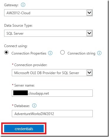
2) Create a new Data Source on top of the previously created Gateway as described here: Create a Data Source and Enable OData Feed in Power BI Admin Center

Here you will usually receive an error when you want to enter credentials for the SQL Database:
AdminCenter_DS

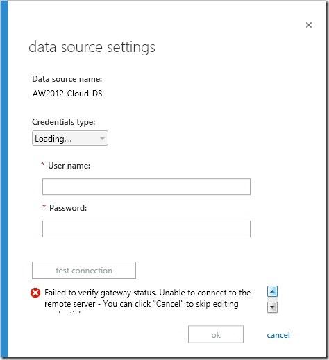
By Clicking on the [credentials]-button a new window pops up. Please note that this is a click-once application that actually runs on your client and is independent of your actual browser!
DataSource_Error

If the Gateway is running on an Azure VM, or basically any machine which cannot be reached from your current client you will receive an error that a connection could not be established or something similar.
Assuming you called your Azure VM “MyCloudServer” and is perfectly reachable via “MyCloudServer.cloudapp.net” you will receive an error saying that “MyCloudServer” (without “.cloudapp.net”) could not be resolved. Which is actually true as the correct server would be “MyCloudServer.cloudapp.net”. Unfortunatelly, this server name cannot be changed anywhere as far as I know. As the name cannot be changed we need to make the name somehow “resolveable”. Bryan manually modifies the hosts file and makes “MyCloudServer” point to the public IP address of “MyCloudServer.cloudapp.net”. This should usually work just fine, but somehow did not work for me. Also the public IP address may change if you reboot your Azure VM and so you would need to modify the hosts-file again.

So these are the findings we mad so far:
– the Data Source Manager is a click-once application which runs on the client
– the client must be able to resolve “MyCloudServer”

After some thinking I ended up with the following:
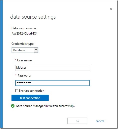
The only machine in my scenario that can correctly resolve “MyCloudServer” is the Azure VM itself! So instead of running the Data Source Manager on my client I simply connected to the Power BI Admin Center from my server and repeated the steps from above there.
Now everything works fine and we can proceed:
DataSource_Success
This connectivity check is only done once and has no further impact (I am not 100% sure on this Smile ). Though, the Username and Password are stored and used for all subsequent connection through the gateway, e.g. for OData access so make sure the user has the necessary access rights.

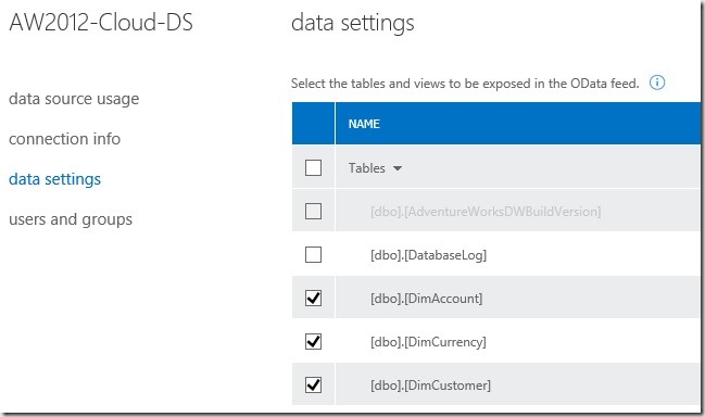
In the next step you can select the tables and views that you want to expose:
DataSource_TablesViews

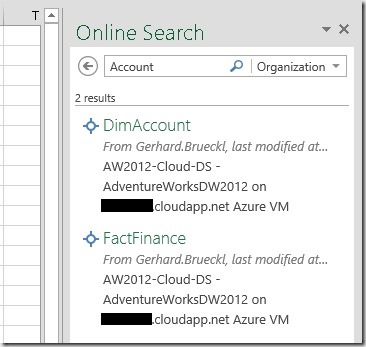
Those can then be searched and queried using Excel and Power Query from any client:
Excel_PowerQuery

And that’s it – The simple trick is to run the Power BI Admin Center from the server itself and create the data source there!

Hope this helps everyone who is dealing with the same issue or wants to setup a demo environment too.

Scheduled Data Refresh of OData Sources in Power BI

With the recent public release of Power BI it is finally possible to refresh Power Pivot workbooks online.Once a workbook is uploaded to SharePoint online and “Enabled” for Power BI you can schedule an automatic data refresh for the Power Pivot model. Though, at the moment only a very limit number of data sources are supported:

  • Windows Azure SQL Database data
  • Open Data protocol (OData) feeds
  • On premises data sources that are enabled for access in Power BI for Office 365

Especially for public available data OData feeds are very popular, for example from Wikipedia. Those public data feeds usually do not require any authentication so one would expect these data sources to work flawless with a scheduled data refresh of Power BI. Well, you are wrong here!
When you create a simple Power Pivot model with one OData source to e.g. Wikipedia, publish it and setup scheduled data refresh you will receive the following error:

Refresh_Error

The error message itself does not reveal any insights on the actual error. If you are in the (more or less) lucky situation that you are also owner of that site you can go to the Power BI Admin Center to get some further details on the error:

AdminCenter_ErrorLog

By downloading the CSV or hovering over a single Message you can see the details:

  1. "Failed to find a match for the data source (connection string: data source=http://publicdata.clouddatahub.net/Web/Tables/fa9af6681cd64206b3aafe6d12408117/V1/Data;include atom elements=Auto;include expanded entities=False;integrated security=SSPI;persist security info=false;time out=600;schema sample size=25;retry count=5;retry sleep=100;keep alive=False;max received message size=4398046511104;base url=http://publicdata.clouddatahub.net/Web/Tables/fa9af6681cd64206b3aafe6d12408117/V1/Data) for the user 'Gerhard.Brueckl@XYZ.onmicrosoft.com'. The user is unauthorized or, the corresponding data source is not created. Check the user's permission to the data source or create a data source for the connection string. Tracing ID: 23f244ad-7921-48f7-b13a-ef68e8cf5503"

It says that for my user no corresponding data source exists or I do not have permissions to access it.

In our case the reason is that our user is unauthorized – the actually data source that was used must not necessarily exist in the user’s data sources (Those can be found via “My Power BI”) for scheduled data refresh to work.

So you will ask yourself what could go possibly wrong here as you are just accessing a public OData feed?!?
The reason is that in the connection string the “Integrated Security”-property is set to SSPI by default. In your local Excel/Power Pivot model this works just fine as the SSPI context can be resolved and sent to the OData feed. Sure the OData feed actually ignores this information as it is public but from an authentication point of view everything works correctly!

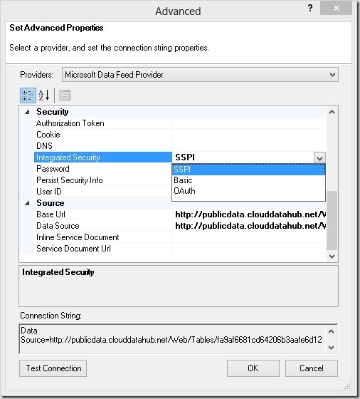
The problem with Scheduled Data Refresh is that SSPI simply does not work as it cannot be resolved and Power BI cannot use any service user for your request if SSPI is defined. The first thing that comes to your mind would be to simply set the authentication method to “Anonymous” which would be perfectly fine for a public data feed. However, Power Pivot does not support Anonymous authentication for OData sources:

OData_Authentication

As SSPI does not work we need to use “Basic” here and provide “User ID” and “Password”. Which UserID/Password you may ask? – and the simple answer is: “It does not matter!”
You can provide any values here, in my case I used “random” for both, User ID and Password! Another thing you need to ensure is that “Persist Securtiy Info” is set to True so your “Password” is stored in the final connection string making Power BI think that authentication is defined correctly within the connection string and Power BI does not have to do anything.

Once you changes those settings your data refresh will work like a charm:

Refresh_Success

On last thing you may realize is the “Running Time”. It takes significantly longer when doing the refresh in Power BI opposed to doing the refresh locally. Just keep that in mind, especially for bigger data feeds.

In the future I hope that Microsoft will introduce some kind of “Anonymous” authentication within the dropdown of Power Pivot or simply check at some point if the OData feed requires any authentication at all hence overwriting the authentication mode specified in the connection string when refreshing.

Applied Basket Analysis in Power Pivot using DAX

Basket Analysis is a very common analysis especially for online shops. Most online shops make use of it to make you buy products that “Others also bought …”. Whenever you view a specific product “Product A” from the online shop, basket analysis allows the shop to show you further products that other customers bought together with “Product A”. Its basically like taking a look into other customers shopping baskets. In this blog post I will show how this can be done using Power Pivot. Alberto Ferrari already blogged about it here some time ago and showed a solution for Power Pivot v1. There is also dedicated chapter in the whitepaper The Many-to-Many Revolution 2.0 which deals with Basket Analysis, already in Power Pivot v2. Power Pivot v2 already made the formula much more readable and also much faster in terms of performance. Though, there are still some things that I would like to add.

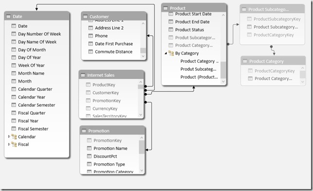
Lets take a look at the initial data model first:Model_Old

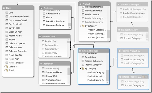
First of all we do not want to modify this model but just extend it so that all previously created measures, calculations and, most important, the reports still work. So the only thing we do is to add our Product-tables again but with a different name. Note that I also added the Subcategory and Category tables in order to allow Basket Analysis also by the Product-Category hierarchy. As we further do not want to break anything we only use an inactive relationship to our ‘Internet Sales’ fact table.

After adding the tables the model looks as follows:Model_New

The next and actually last thing to do is to add the following calculated measure:

Sold in same Order :=
CALCULATE (
COUNTROWS ( ‘Internet Sales’ ),
CALCULATETABLE (
SUMMARIZE (
‘Internet Sales’,
‘Internet Sales’[Sales Order Number]
),
ALL ( ‘Product’ ),
USERELATIONSHIP ( ‘Internet Sales’[ProductKey], ‘Filtered Product’[ProductKey] )
)
)

(formatted using DAX Formatter)

The inner CALCULATETABLE returns a list/table of all [Sales Order Numbers] where a ‘Filtered Product’ was sold and uses this table to extend the filter on the ‘Internet Sales’ table. It is also important to use ALL(‘Product’) here otherwise we would have two filters on the same column ([ProductKey]) which would always result in an empty table. Doing a COUNTROWS finally returns all for all baskets where the filtered product was sold.
We could also change ‘Internet Sales'[Sales Order Number] to ‘Internet Sales'[CustomerKey] in order to analyze what other customers bought also in different baskets (This was done for Example 3). The whole SUMMARIZE-function could also be replaced by VALUES(‘Internet Sales'[Sales Order Number]). I used SUMMARIZE here as I had better experiences with it in terms of performance in the past, though, this may depend on your data. The calculation itself also works with all kind of columns and hierarchies, regardless whether its from table ‘Product’, ‘Filtered Product’, or any other table!

So what can we finally do with this neat formula?

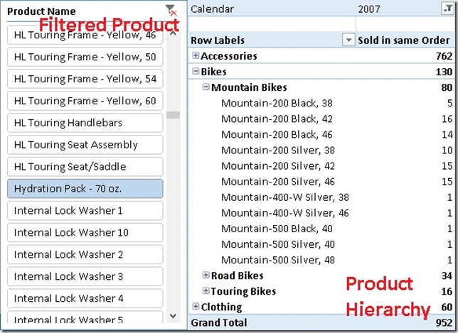
1) Classic Basket Analysis – “Others also bought …”:
Result_ClassicBasketAnalysis

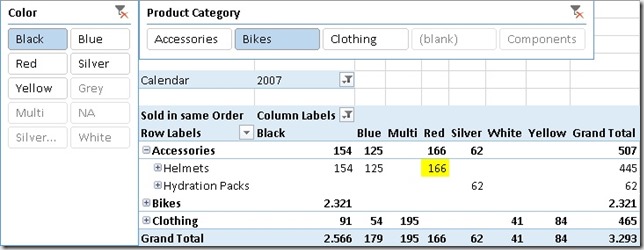
As we can see Hydration Packs are more often sold together with Mountain Bikes opposed to Road Bikes and Touring Bikes. We could also use a slicer on ‘Filtered Product Subcategory’=”Accessories” in order to see how often Accessories are sold together with other products. You may analyze by Color and Product Category:
Result_ByColor
As we can see people that buy black bikes are more likely to buy red helmets than blue helmets.

2) Basket Analysis Matrix:
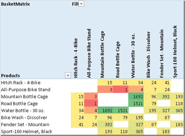
What may also be important for us is which products are sold together the most often? This can be achieved by pulling ‘Product’ on rows and ‘Filtered Product’ on columns. By further applying conditional formatting we can identify correlations pretty easy:
Result_BasketMatrix
Water Bottles are very often sold together with Bottle Cages – well, not really a surprise. Again, you can also use all kind of hierarchies here for your analysis.
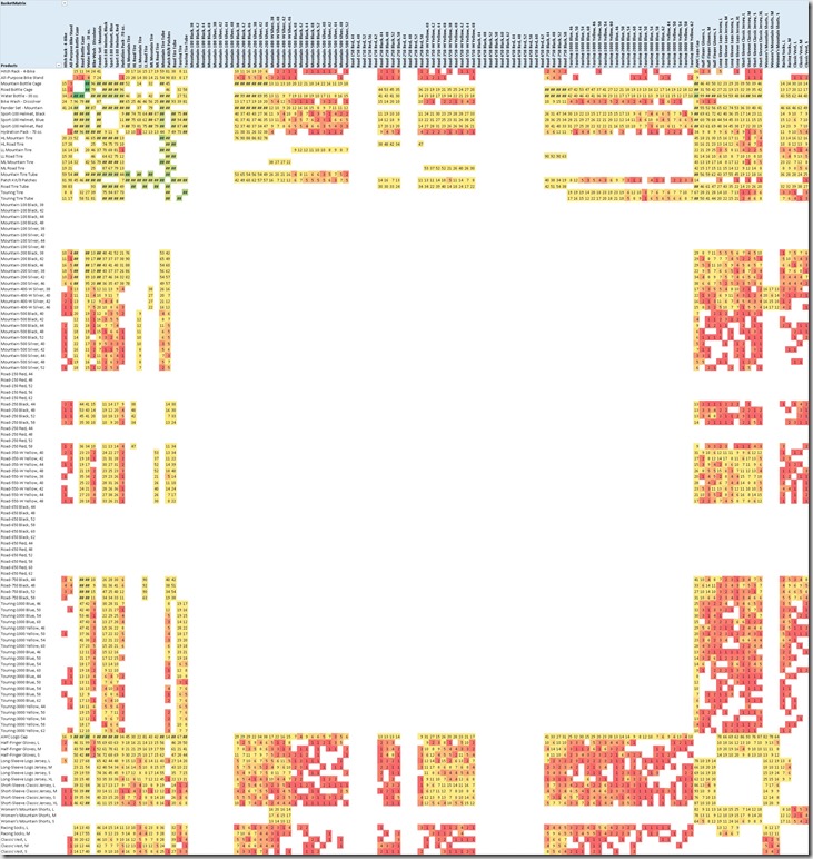
This is what the whole matrix looks like:
Result_BasketMatrixFull
The big blank section in the middle are our Bikes. This tells us that there is no customer that bought two bikes in the same order/basket.

For this analysis I used an extended version of the calculation above to filter out values where ‘Product’ = ‘Filtered Product’ as of course every product is sold within its own basket:

BasketMatrix :=
IF (
MIN ( ‘Product’[ProductKey] )
<> MIN ( ‘Filtered Product’[ProductKey] ),
[Sold in same Order]
)

3) Find Customers that have not bough a common product yet
As we now know from the above analysis which products are very often bought together we can also analyze which customers do not fall in this pattern – e.g. customers who have bough a Water Bottle but have not bought a Bottle Cage yet. Again we can extend our base-calculation to achieve this:

Not Sold to same Customer :=
IF (
NOT ( ISBLANK ( [Sum SA] ) ) && NOT ( [Sold to same Customer] ),
“Not Sold Yet”
)

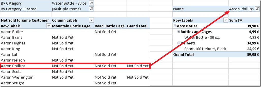
The first part checks if the selected ‘Product’ was sold to the customer at all and the second part checks if the ‘Filtered Product’ was not sold to the customer yet. In that case we return “Not Sold Yet”, and otherwise  BLANK() which is the default if the third parameter is omitted. That’s the result:
Result_NotSoldToCustomer
Aaron Phillips has bought a Water Bottle but no Mountain Bottle Cage nor a Road Bottle Cage – maybe we should send him some advertisement material on Bottle Cages? Smile


As you can see there are a lot of analyses possible on top of that little measure that we created originally. All work with any kind of grouping or hierarchy that you may have and no change to your data model is necessary, just a little extension.

And that’s it – Basket Analysis made easy using Power Pivot and DAX!

Downloads:

Sample Excel Workbook with all Examples: BasketAnalysis.xlsx
Sample PowerBI Desktop file with all Examples (DAX only, no Visuals): BasketAnalysis.pbix

Optimizing Columnar Storage for Measures

First of all I have to thank Marco Russo for his blog post on Optimizing High Cardinality Columns in Vertipaq and also his great session at SQL PASS Rally Nordic in Stockholm last year which taught me a lot about columnar storage in general. I highly recommend everyone to read the two mentioned resources before continuing here. Most of the ideas presented in this post are based on these concepts and require at least basic knowledge in columnar storage.

When writing one of my recent posts I ended up with a Power Pivot model with roughly 40M rows. It contained internet logs from Wikipedia, how often someone clicked on a given page per month and how many bytes got downloaded. As you can imagine those values can vary very heavily, especially the amount of bytes downloaded. So in the Power Pivot model we end up having a lot of distinct values in our column that we use for our measure. As you know from Marcos posts, the allocated memory and therefore also the  performance of columnar storage systems is directly related to the number of distinct values in a column – the more the worse. Marco already described an approach to split up a single column with a lot of distinct values into several columns with less distinct values to optimize storage. These concepts can also be used on columns that contain measures or numeric values in general. Splitting numeric values is quite easy, assuming your values range from 1 to 1,000,000 you can split this column into two by dividing the value by 1000 and using MOD 1000 for the second column. Instead of one column with the value 123,456 you end up with two columns with the values 123 and 456. In terms of storage this means that instead of 1,000,000 distinct values we only need to store 2 x 1,000 distinct values. Nothing new so far.

The trick is to combine those columns again at query time to get the original results as before the split. For some aggregations like SUM this is pretty straight forward, others are a bit more tricky. Though, in general the formulas are not really very complex and can be adopted very easily to handle any number of columns:

Aggregation DAX Formula
Value_SUM1 =SUMX(‘1M_Rows_splitted’, [Value_1000] * 1000 + [Value_1])
Value_SUM2 =SUM ( ‘1M_Rows_splitted'[Value_1000] ) * 1000
    + SUM ( ‘1M_Rows_splitted'[Value_1] )
Value_MAX =MAXX(‘1M_Rows_splitted’, [Value_1000] * 1000 + [Value_1])
Value_MIN =MINX(‘1M_Rows_splitted’, [Value_1000] * 1000 + [Value_1])
Value_COUNT =COUNTX(‘1M_Rows_splitted’, [Value_1000] * 1000 + [Value_1])
Value_DISTINCTCOUNT =COUNTROWS (
    SUMMARIZE (
        ‘1M_Rows_splitted’,
        ‘1M_Rows_splitted'[Value_1000],
        ‘1M_Rows_splitted'[Value_1]))

As you can see you can still mimic most kind of aggregation even if the [Value]-column is split up.

Though, don’t exaggerate splitting your columns – too many may be a bit inconvenient to handle and may neglect the effect resulting in worse performance. Marco already showed that you can get a reduction of up to 90% in size, during my simple tests I came up with about the same numbers. Though, it very much depends on the number of distinct values that you actually have in your column!

I would not recommend to always use this approach for all your measure column – no, definitely not! First check how many distinct values your data/measures contain and decide afterwards. For 1 million distinct values it is probably worth it, for 10,000 you may reconsider using this approach. Most important here is to test this pattern with your own data, data model and queries! Test it in terms of size and of course also in terms of performance. It may be faster to split up columns but it may also be slower and it may be also different for each query that you execute against the tabular model / Power Pivot. Again, test with your own data, data model and queries to get representative results! 

Here is a little test that you may run on your own to test this behavior. Simple create the following Power Query using M, load the result into Power Pivot and save the workbook. It basically creates a table with 1 million distinct values (0 to 999,999) and splits this column up into two. You can just copy the workbook, remove the last step “Remove Columns” and save it again to get the “original” workbook and Power Pivot model.

let
    List1 = List.Numbers(0, 1000000),

    TableFromList = Table.FromList(List1, Splitter.SplitByNothing(), null, null, ExtraValues.Error),
    RenamedColumns = Table.RenameColumns(TableFromList,{{"Column1", "Value"}}),
    ChangedType1 = Table.TransformColumnTypes(RenamedColumns,{{"Value", type number}}),
    InsertedCustom = Table.AddColumn(ChangedType1, "Value_1000", each Number.RoundDown([Value] / 1000)),
    InsertedCustom1 = Table.AddColumn(InsertedCustom, "Value_1", each Number.Mod([Value], 1000)),
    ChangedType = Table.TransformColumnTypes(InsertedCustom1,{{"Value_1000", type number}, {"Value_1", type number}}),
    RemovedColumns = Table.RemoveColumns(ChangedType,{"Value"})
in
    RemovedColumns

This is what I ended up with when you compare those two workbooks:

  # distinct values Final Size
single column 1,000,000 14.4 MB
two columns 2 x 1,000 1.4 MB

We also get a reduction in size of 90%! Though, this is a special scenario …
In the real world, taking my previous scenario with the Wikipedia data as an example, I ended up with a reduction to 50%, still very good though. But as you can see the reduction factor varies very much.

Downloads:

Sample workbook with Power Query: 1M_Rows_splitted.xlsx

Upcoming Conferences and Events in Q1 2013

After PASS SQL Rally Nordic in Stockholm last year I am very happy to announce that I am going to speak at two more events in the first quarter of 2013.

SQLKonferenz2014
I will do a session at the “Deutsche SQL Server Konferenz 2014” (=”German SQL Server Conference 2014″) on “Big Data Scenario mit Power BI vs. SAP HANA“. It is basically an advanced version of my blog post on SAP HANAs Big Data Scenario with Power BI with much more insights details on both technologies. The conference itself is a 3 day conference from 10th to 12th of February where day 1 is reserved for pre-conference sessions. It also features a lot of international speakers and of course also a good amount of English sessions (mine will be in German though). Also my colleague Marcel Franke will do a session about PDW and R which you also do not want to miss if you are into Big Data and predictive analytics!
Check out the agenda and make sure you register in time!

SQLSaturdayBanner
Later on the 6th of March I will speak at the SQLSaturday #280 in Vienna on “Scaling Analysis Services in the Cloud“. (This is not a typo, its really on 6th of March which is actually a Thursday!) The session focuses on how to get the best performance out of multidimensional Analysis Services solutions when they are moved to the Windows Azure cloud. In the end I will come up with some best practices and guide lines for this and similar scenarios.
Just make sure that you register beforehand to enjoy this full day of free sessions and trainings!

Hope to see you there!