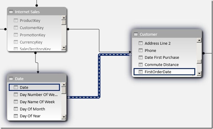
In my previous post I showed a new approach on how to calculate new (and returning) customers in PowerPivot/tabular using DAX. We ended up with a solution where we added the customers first order date as a calculated column to our customer-table. This column was then linked to our date-table with an inactive relationship. The final calculation used USERELATIONSHIP() to make use of this relationship as follows:
COUNTROWS(Customer),
USERELATIONSHIP(Customer[FirstOrderDate], ‘Date’[Date]))
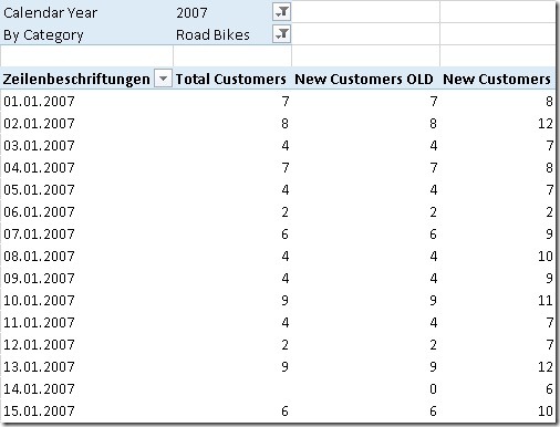
This calculation performs really well as it does not have to touch the fact-table to get the count of new customers. And this is also the issue with the calculation as other filters are not reflected in the calculation:
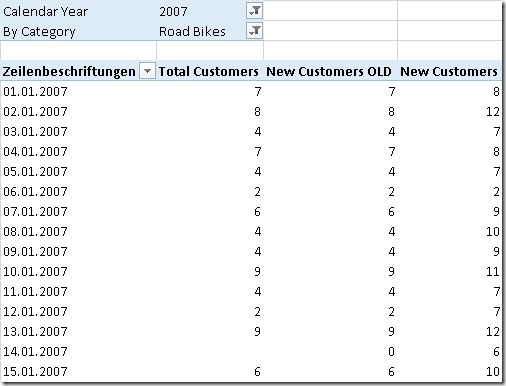
Take row 2 as an example: we have 8 “Total Customers” of which 12 are “New Customers”. Obviously an error in the calculation. The PivotTable is filtered to Category=”Road Bikes” and we have 8 customers on the 2nd of February that bought a road bike. The “New Customers” calculation on the other hand is not related to the Subcategory and shows 12 as in total there were 12 new customers for all products.
To get our calculation working also with other filters we have to somehow relate it to our fact-table. So far we calculated the customers first order date only in the customer table. The customers first order may be related to several fact-rows, e.g. one row for each product the customer bought. Our “New Customers” calculation should only include customers that are active considering also all other filters.
To identify a customers first order in our fact-table we can again use a calculated column and also re-use our previous calculated column in our Customer-table that holds the customers first order date:
ISBLANK(
LOOKUPVALUE(
Customer[CustomerKey],
Customer[CustomerKey],
[CustomerKey],
Customer[FirstOrderDate],
[Order Date]
)))
This returns True for all fact-rows associated with a customers first order and False for all other rows.
The final “New Customers v2” calculation is quite simple then – in addition to the active filters we add a further filter to only select rows that are associated to a customers first order:
[Total Customers],
‘Internet Sales’[IsCustomersFirstOrder] = TRUE())
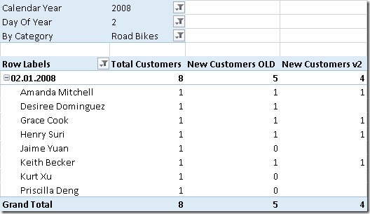
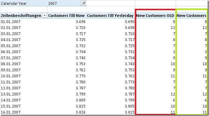
And this are the results:
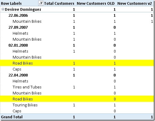
As you can see there are still differences between “New Customers OLD” and “New Customers v2”. But is this really a problem with the new calculation? Lets analyze the issue taking customer “Desiree Dominguez” where we encounter the first difference as an example:
“Desiree Dominguez” had her first order on the 22th of June in 2006. So she is actually no “new customer” in 2008. The reason why the old calculation counts her as “new customer” is that it was the first time that she bought a product of subcategory “Road Bikes”. Whether this is correct or not is up to your business definition of a “new customer”. According to my experience it is more likely that “Desiree Dominguez” is not counted as a new customer in 2008 and so the “New Customer v2” actually returns the more accurate results.
Additional stuff:
An other option for this calculation is to rank the [Order Date] or [Sales Order Number] for each customer within the fact-table using the calculation below:
FILTER(
ALL(‘Internet Sales’),
[CustomerKey] = EARLIER([CustomerKey])),
[Order Date],
[Order Date],
1,
DENSE
)
[Order Date] could be replaced by [Sales Order Number]. This makes sense if a customer can have multiple orders per day and you also want to distinguish further by [Sales Order Number]. The new field would also allow new analysis. For example the increase/decrease in sales from the second order compared to the first order and so on.
The “New Customer” calculation in this case would still be similar. We just have to filter on the new calculated column instead:
[Total Customers],
‘Internet Sales’[CustomersOrderNr] = 1)
Download Final Model (Office 2013!)
The multidimensional model:
The whole logic of extending the fact-table to identify rows that can be associated with a customers first order can also be used in a multidimensional model. Once we prepared the fact-table accordingly the calculations are quite easy. The biggest issues here does not reside in the multidimensional model itself but in the ETL/relational layer as this kind of operation can be quite complex – or better say time-consuming in terms of ETL time.
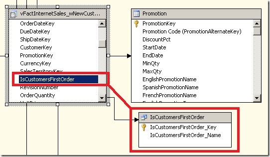
At this point I will not focus on the necessary ETL steps but start with an already prepared fact-table and highlight the extensions that have to be made in the multidimensional model. The fact-table already got extended by a new column called [IsCustomersFirstOrder] similar to the one we created in tabular using a DAX calculated column. It has a value of 1 for rows associated with a customers first order and 0 for all other rows.
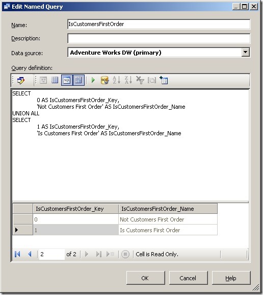
The next thing we have to do is to create a new table in our DSV to base our new dimension on. For simplicity I used this named query:
This table is then joined to the new fact-table:
The new dimension is quite simple as it only contains one attribute:
You may hide the whole dimension in the end as it may only be used to calculate our “new customers” and nowhere else and may only confuse the end-user.
Once we have added the dimension also to our cube we can create a new calculated measure to calculate our “new customers” as follows:
[Measures].[Customer Count],
[Is Customers First Order].[Is Customers First Order].&[1]
), ASSOCIATED_MEASURE_GROUP = ‘Internet Customers’
, FORMAT_STRING = ‘#,##0’;
The calculation is based on the existing [Customer Count]-measure which uses DistinctCount-aggregation. Similar to DAX with just extend the calculation by further limiting the cube-space where “Is customers First Order” = 1.
This approach also allows you to create aggregations if necessary to further improve performance. So this is probably also the best way in terms of query-performance to calculate the count of new customers in a multidimensional model.
