In my last post I described and approach on how to calculate consolidated values (adjusted by intercompany eliminations) using PowerPivot and DAX. In this post I will extend this technique so it can also be used with parallel hierarchies as this is also very common in financial applications.
Switching from a single hierarchy to multiple parallel hierarchies has several drawbacks for tabular models:
1) business keys cannot be used to build the PC-hierarchy as they are not unique anymore
2) artificial keys and parent-keys are required
3) as business keys are not unique anymore, we also cannot create a relationship between facts and our dimension
4) PowerPivot tables do not support “UNION” to load several single hierarchies and combine them
All the issues described above have to be handled before the hierarchies can be loaded into PowerPivot. This is usually done in a relational database but this will not be covered in this post.
For simplicity I created a table in Excel that already has the correct format:
| ID | ParentID | SenderID | Name |
| 1 | TOT | My Whole Company by Region | |
| 2 | 1 | EUROPE | Europe |
| 3 | 2 | GER | Germany Company |
| 4 | 2 | FR | French Company |
| 5 | 1 | NA | North America |
| 6 | 5 | USA | US Company |
| 7 | 5 | CAN | Canadian Company |
| -99 | EXTERNAL | EXTERNAL | |
| 8 | TOT_2 | My Whole Company Legal View | |
| 9 | 8 | JV | Joint Ventures |
| 10 | 9 | FR | French Company |
| 11 | 9 | USA | US Company |
| 12 | 8 | HOLD | My cool Holding |
| 13 | 12 | GER | Germany Company |
| 14 | 12 | CAN | Canadian Company |
We have 2 parallel hierarchies – “My Whole Company by Region” and “My Whole Company Legal View”. In PowerPivot this looks like this:

As I already noted above, the SenderIDs are not unique anymore, and therefore we cannot create a relationship to our fact-table. So we have to handle this in our calculation. The approach is similar to handling SCD2 dimensions in PowerPivot what I described in previous posts (Part1 and Part2). We use CONTAINS-function to filter our fact-table based on the currently active SenderIDs in the dimension-table:
Value_Sender:=
CALCULATE([Value_SUM],
FILTER(
     'Facts',
     CONTAINS(
          'Sender',
          'Sender'[SenderID],
          'Facts'[SenderID]))
)
Actually this is the only difference in the calculation when we are dealing with multiple parallel hierarches. The other calculations are the same with the only difference that we have to use [Value_Sender] instead of [Value_SUM]:
Value_Internal:=
 CALCULATE([Value_Sender],
 FILTER(
      'Facts',
      CONTAINS(
           'Sender',
           'Sender'[SenderID],
           'Facts'[ReceiverID]))
 )
and
Value_External:=
 CALCULATE([Value_Sender],
 FILTER(
      'Facts',
      NOT(
           CONTAINS(
                'Sender',
                'Sender'[SenderID],
                'Facts'[ReceiverID])))
 )
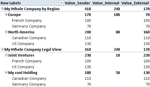
As you can see this approach also works very well with multiple hierarchies. In the end we get the desired results:

Taking a look at “My cool Holding” we see that a value of 50 is eliminated as there have been sales from CAN to GER. On top-level of the hierarchy we see the same values being eliminated (170) as both hierarchies contain the same companies and therefore only sales to EXTERNAL can summed up to get the correct value.
As this technique operates on leaf-level it works with all possible hierarchies regardless of how many companies are assigned to which node or how deep the hierarchies are!
(Just to compare the values from above – the fact-table is the same as in the previous post: )
| SenderID | ReceiverID | Value |
| FR | GER | 100 |
| CAN | GER | 50 |
| GER | EXTERNAL | 70 |
| USA | CAN | 30 |
| USA | FR | 10 |
| USA | EXTERNAL | 90 |
| CAN | USA | 50 |
| CAN | EXTERNAL | 10 |