Applied Basket Analysis in Power Pivot using DAX

Basket Analysis is a very common analysis especially for online shops. Most online shops make use of it to make you buy products that “Others also bought …”. Whenever you view a specific product “Product A” from the online shop, basket analysis allows the shop to show you further products that other customers bought together with “Product A”. Its basically like taking a look into other customers shopping baskets. In this blog post I will show how this can be done using Power Pivot. Alberto Ferrari already blogged about it here some time ago and showed a solution for Power Pivot v1. There is also dedicated chapter in the whitepaper The Many-to-Many Revolution 2.0 which deals with Basket Analysis, already in Power Pivot v2. Power Pivot v2 already made the formula much more readable and also much faster in terms of performance. Though, there are still some things that I would like to add.

Lets take a look at the initial data model first:Model_Old
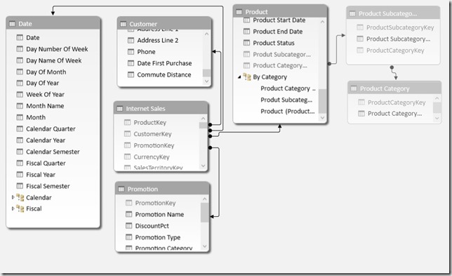
First of all we do not want to modify this model but just extend it so that all previously created measures, calculations and, most important, the reports still work. So the only thing we do is to add our Product-tables again but with a different name. Note that I also added the Subcategory and Category tables in order to allow Basket Analysis also by the Product-Category hierarchy. As we further do not want to break anything we only use an inactive relationship to our ‘Internet Sales’ fact table.

After adding the tables the model looks as follows:Model_New
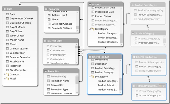
The next and actually last thing to do is to add the following calculated measure:

Sold in same Order :=
CALCULATE (
COUNTROWS ( ‘Internet Sales’ ),
CALCULATETABLE (
SUMMARIZE (
‘Internet Sales’,
‘Internet Sales’[Sales Order Number]
),
ALL ( ‘Product’ ),
USERELATIONSHIP ( ‘Internet Sales’[ProductKey], ‘Filtered Product’[ProductKey] )
)
)

(formatted using DAX Formatter)

The inner CALCULATETABLE returns a list/table of all [Sales Order Numbers] where a ‘Filtered Product’ was sold and uses this table to extend the filter on the ‘Internet Sales’ table. It is also important to use ALL(‘Product’) here otherwise we would have two filters on the same column ([ProductKey]) which would always result in an empty table. Doing a COUNTROWS finally returns all for all baskets where the filtered product was sold.
We could also change ‘Internet Sales'[Sales Order Number] to ‘Internet Sales'[CustomerKey] in order to analyze what other customers bought also in different baskets (This was done for Example 3). The whole SUMMARIZE-function could also be replaced by VALUES(‘Internet Sales'[Sales Order Number]). I used SUMMARIZE here as I had better experiences with it in terms of performance in the past, though, this may depend on your data. The calculation itself also works with all kind of columns and hierarchies, regardless whether its from table ‘Product’, ‘Filtered Product’, or any other table!

So what can we finally do with this neat formula?

1) Classic Basket Analysis – “Others also bought …”:
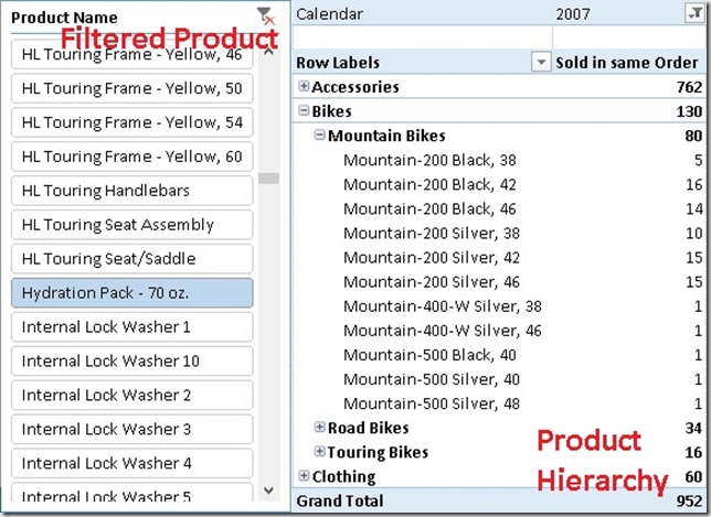
Result_ClassicBasketAnalysis

As we can see Hydration Packs are more often sold together with Mountain Bikes opposed to Road Bikes and Touring Bikes. We could also use a slicer on ‘Filtered Product Subcategory’=”Accessories” in order to see how often Accessories are sold together with other products. You may analyze by Color and Product Category:
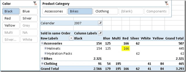
Result_ByColor
As we can see people that buy black bikes are more likely to buy red helmets than blue helmets.

2) Basket Analysis Matrix:
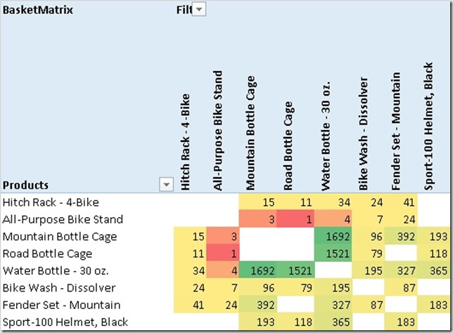
What may also be important for us is which products are sold together the most often? This can be achieved by pulling ‘Product’ on rows and ‘Filtered Product’ on columns. By further applying conditional formatting we can identify correlations pretty easy:
Result_BasketMatrix
Water Bottles are very often sold together with Bottle Cages – well, not really a surprise. Again, you can also use all kind of hierarchies here for your analysis.
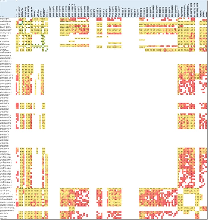
This is what the whole matrix looks like:
Result_BasketMatrixFull
The big blank section in the middle are our Bikes. This tells us that there is no customer that bought two bikes in the same order/basket.

For this analysis I used an extended version of the calculation above to filter out values where ‘Product’ = ‘Filtered Product’ as of course every product is sold within its own basket:

BasketMatrix :=
IF (
MIN ( ‘Product’[ProductKey] )
<> MIN ( ‘Filtered Product’[ProductKey] ),
[Sold in same Order]
)

3) Find Customers that have not bough a common product yet
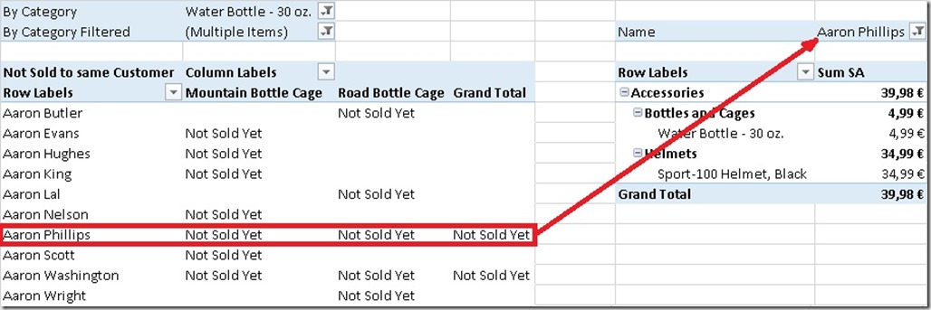
As we now know from the above analysis which products are very often bought together we can also analyze which customers do not fall in this pattern – e.g. customers who have bough a Water Bottle but have not bought a Bottle Cage yet. Again we can extend our base-calculation to achieve this:

Not Sold to same Customer :=
IF (
NOT ( ISBLANK ( [Sum SA] ) ) && NOT ( [Sold to same Customer] ),
“Not Sold Yet”
)

The first part checks if the selected ‘Product’ was sold to the customer at all and the second part checks if the ‘Filtered Product’ was not sold to the customer yet. In that case we return “Not Sold Yet”, and otherwise  BLANK() which is the default if the third parameter is omitted. That’s the result:
Result_NotSoldToCustomer
Aaron Phillips has bought a Water Bottle but no Mountain Bottle Cage nor a Road Bottle Cage – maybe we should send him some advertisement material on Bottle Cages? Smile


As you can see there are a lot of analyses possible on top of that little measure that we created originally. All work with any kind of grouping or hierarchy that you may have and no change to your data model is necessary, just a little extension.

And that’s it – Basket Analysis made easy using Power Pivot and DAX!

Downloads:

Sample Excel Workbook with all Examples: BasketAnalysis.xlsx
Sample PowerBI Desktop file with all Examples (DAX only, no Visuals): BasketAnalysis.pbix

Optimizing Columnar Storage for Measures

First of all I have to thank Marco Russo for his blog post on Optimizing High Cardinality Columns in Vertipaq and also his great session at SQL PASS Rally Nordic in Stockholm last year which taught me a lot about columnar storage in general. I highly recommend everyone to read the two mentioned resources before continuing here. Most of the ideas presented in this post are based on these concepts and require at least basic knowledge in columnar storage.

When writing one of my recent posts I ended up with a Power Pivot model with roughly 40M rows. It contained internet logs from Wikipedia, how often someone clicked on a given page per month and how many bytes got downloaded. As you can imagine those values can vary very heavily, especially the amount of bytes downloaded. So in the Power Pivot model we end up having a lot of distinct values in our column that we use for our measure. As you know from Marcos posts, the allocated memory and therefore also the  performance of columnar storage systems is directly related to the number of distinct values in a column – the more the worse. Marco already described an approach to split up a single column with a lot of distinct values into several columns with less distinct values to optimize storage. These concepts can also be used on columns that contain measures or numeric values in general. Splitting numeric values is quite easy, assuming your values range from 1 to 1,000,000 you can split this column into two by dividing the value by 1000 and using MOD 1000 for the second column. Instead of one column with the value 123,456 you end up with two columns with the values 123 and 456. In terms of storage this means that instead of 1,000,000 distinct values we only need to store 2 x 1,000 distinct values. Nothing new so far.

The trick is to combine those columns again at query time to get the original results as before the split. For some aggregations like SUM this is pretty straight forward, others are a bit more tricky. Though, in general the formulas are not really very complex and can be adopted very easily to handle any number of columns:

Aggregation DAX Formula
Value_SUM1 =SUMX(‘1M_Rows_splitted’, [Value_1000] * 1000 + [Value_1])
Value_SUM2 =SUM ( ‘1M_Rows_splitted'[Value_1000] ) * 1000
    + SUM ( ‘1M_Rows_splitted'[Value_1] )
Value_MAX =MAXX(‘1M_Rows_splitted’, [Value_1000] * 1000 + [Value_1])
Value_MIN =MINX(‘1M_Rows_splitted’, [Value_1000] * 1000 + [Value_1])
Value_COUNT =COUNTX(‘1M_Rows_splitted’, [Value_1000] * 1000 + [Value_1])
Value_DISTINCTCOUNT =COUNTROWS (
    SUMMARIZE (
        ‘1M_Rows_splitted’,
        ‘1M_Rows_splitted'[Value_1000],
        ‘1M_Rows_splitted'[Value_1]))

As you can see you can still mimic most kind of aggregation even if the [Value]-column is split up.

Though, don’t exaggerate splitting your columns – too many may be a bit inconvenient to handle and may neglect the effect resulting in worse performance. Marco already showed that you can get a reduction of up to 90% in size, during my simple tests I came up with about the same numbers. Though, it very much depends on the number of distinct values that you actually have in your column!

I would not recommend to always use this approach for all your measure column – no, definitely not! First check how many distinct values your data/measures contain and decide afterwards. For 1 million distinct values it is probably worth it, for 10,000 you may reconsider using this approach. Most important here is to test this pattern with your own data, data model and queries! Test it in terms of size and of course also in terms of performance. It may be faster to split up columns but it may also be slower and it may be also different for each query that you execute against the tabular model / Power Pivot. Again, test with your own data, data model and queries to get representative results! 

Here is a little test that you may run on your own to test this behavior. Simple create the following Power Query using M, load the result into Power Pivot and save the workbook. It basically creates a table with 1 million distinct values (0 to 999,999) and splits this column up into two. You can just copy the workbook, remove the last step “Remove Columns” and save it again to get the “original” workbook and Power Pivot model.

let
    List1 = List.Numbers(0, 1000000),

    TableFromList = Table.FromList(List1, Splitter.SplitByNothing(), null, null, ExtraValues.Error),
    RenamedColumns = Table.RenameColumns(TableFromList,{{"Column1", "Value"}}),
    ChangedType1 = Table.TransformColumnTypes(RenamedColumns,{{"Value", type number}}),
    InsertedCustom = Table.AddColumn(ChangedType1, "Value_1000", each Number.RoundDown([Value] / 1000)),
    InsertedCustom1 = Table.AddColumn(InsertedCustom, "Value_1", each Number.Mod([Value], 1000)),
    ChangedType = Table.TransformColumnTypes(InsertedCustom1,{{"Value_1000", type number}, {"Value_1", type number}}),
    RemovedColumns = Table.RemoveColumns(ChangedType,{"Value"})
in
    RemovedColumns

This is what I ended up with when you compare those two workbooks:

  # distinct values Final Size
single column 1,000,000 14.4 MB
two columns 2 x 1,000 1.4 MB

We also get a reduction in size of 90%! Though, this is a special scenario …
In the real world, taking my previous scenario with the Wikipedia data as an example, I ended up with a reduction to 50%, still very good though. But as you can see the reduction factor varies very much.

Downloads:

Sample workbook with Power Query: 1M_Rows_splitted.xlsx