Excel CUBE-Functions and MDX UniqueNames

Two weeks ago at the German SQL Server Conference 2015 I was at Peter Myer’s session about Mastering the CUBE Functions in Excel. (PS: Peter is also speaking on our upcoming SQLSaturday #374 in Vienna next week and at PASS SQLRally in Copenhagen the week after). After his session we had a further discussion about this topic and our experiences on how to use Excels CUBE-functions in order to build nice Dashboards with native Excel functionalities that also work with e.g. Excel Services. Its always great to exchange with people that share the same passion on he same topic! One thing we both agreed on that is missing currently is a way to get the MDX UniqueName of something that is selected in a slicer, filter or simply in a cell using CUBEMEMBER-function. I once used a special Cube Measure which was created in MDX Script which returned the UniqueName of a given member that was selected together with this special measure. For this to work with Excel you need to know how Excel builds the MDX when querying cube values using CUBEVALUE-function. Here is a little example:
Excel_CubeValue_Formula
This produces the following MDX query:

  1. SELECT
  2. {
  3.     (
  4.         [Measures].[Internet Sales Amount],
  5.         [Product].[Category].&[1]
  6.     )
  7. } ON 0
  8. FROM [Adventure Works]
  9. CELL PROPERTIES VALUE, FORMAT_STRING, LANGUAGE, BACK_COLOR, FORE_COLOR, FONT_FLAGS

So it basically creates a tuple that contains everything you pass into the CUBEVALUE-Function as a parameter. Knowing this we can create a calculated measure to get the MDX UniqueName of this tuple using MDX StrToTuple()- and MDX AXIS()-function:

  1. MEMBER [Measures].[Excel TupleToStr] AS (
  2. TupleToStr(axis(0).item(0))
  3. )

Replacing the [Measures].[Internet Sales Amount] of our initial CUBEVALUE-function with this new measure would return this to Excel:

  1. ([Measures].[Internet Sales Amount],[Product].[Category].&[1])


Ok, so far so good but nothing really useful as you need to hardcode the member’s UniqueName into the CUBEVALUE-function anyway so you already know the UniqueName.
However, this is not the case if you are dealing with Pivot Table Page Filters and/or Slicers! You can simply refer to them within the CUBEVALUE-function but you never get the UniqueName of the selected item(s). Well, at least not directly! But you can use the approach described above, using an special MDX calculated measure, to achieve this as I will demonstrate on the next pages.

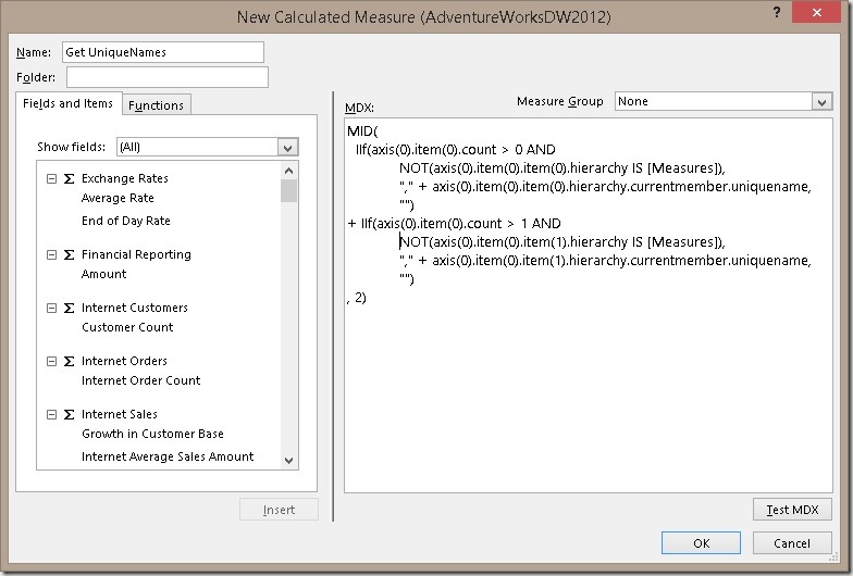
Calculated measures can only be created using the Pivot Table interface but can also be used in CUBE-functions. So first thing you need to do is to create a Pivot Table and add a new MDX Calculated Measure:
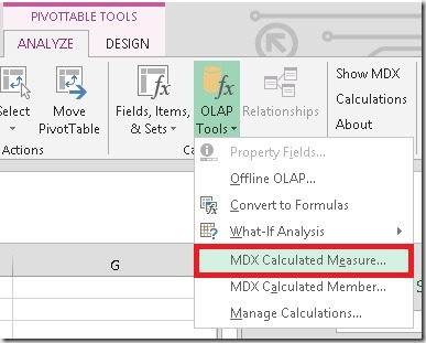
Excel_Create_MDX_calculated_measure

!Caution! some weird MDX coming !Caution!


Excel_Create_MDX_calculated_measure2

You may wonder, why such a complex MDX is necessary and what it actually does. What it does is the following: Based on the example MDX query that Excel generates (as shown above) this is a universal MDX that returns the MDX UniqueName of any other member that is selected together with our measure using the CUBEVALUE-function. It also removes the UniqueName of the measure itself so the result can be used again with any other measure, e.g. [Internet Sales Amount]
The reason why it is rather complex is that Excel may group similar queries and execute them as a batch/as one query to avoid too many executions which would slow down the overall performance. So we cannot just reference the first element of our query as it may belong to any other CUBEVALUE-function. This MDX deals with all this kinds of issues.

The MDX above allows you to specify only two additional filters but it may be extended to any number of filters that you pass in to the CUBEMEMBER-function. This would be the general pattern:

  1. MID(
  2.   IIf(axis(0).item(0).count > 0 AND
  3.         NOT(axis(0).item(0).item(0).hierarchy IS [Measures]),
  4.     "," + axis(0).item(0).item(0).hierarchy.currentmember.uniquename,
  5.     "")
  6. + IIf(axis(0).item(0).count > 1 AND
  7.         NOT(axis(0).item(0).item(1).hierarchy IS [Measures]),
  8.     "," + axis(0).item(0).item(1).hierarchy.currentmember.uniquename,
  9.     "")
  10. + IIf(axis(0).item(0).count > n AND
  11.         NOT(axis(0).item(0).item(n).hierarchy IS [Measures]),
  12.     "," + axis(0).item(0).item(n).hierarchy.currentmember.uniquename,
  13.     "")
  14. , 2)

After creating this measure we can now use it in our CUBE-functions in combination with our filters and slicers:
Excel_MDX_CUBEVALUE_UniqueNames_Filter
Excel_MDX_CUBEVALUE_UniqueNames_Slicer

You may noted that I had to use CUBERANKEDMEMBER here. This is because filters and slicers always return a set and if we would pass in a set to our CUBEVALUE function a different MDX query would be generated which would not allow us to extract the single UniqueNames of the selected items using the approach above (or any other MDX I could think of). So, this approach currently only works with single selections! I hope that the Excel team will implement a native function to extract the UniqueName(s) of the selected items in the future to make this workaround obsolete!

Once we have our UniqeName(s) we can now use them in e.g. a CUBESET-function to return the Top 10 days for a given group of product (filter) and the selected year (slicer):
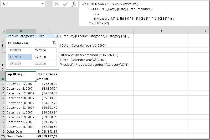
Excel_MDX_CUBESET_TopCount

And that’s it!

So why is this so cool?

  • It works with SSAS (multidimensional and tabular) and Power Pivot as Excel still uses MDX to query all those sources. It may also work with SAP HANA’s ODBO connector but I have not tested this yet!
  • It does not require any VBA which would not work in Excel Services – this solution does!
  • The calculation is stored within the Excel Workbook so it can be easily shared with other users!
  • There is no native Excel functionality which would allow you to create a simple Top 10 report which works with filters and slicers as shown above or any more complex dynamic report/dashboard with any dynamic filtering.

So no more to say here – Have fun creating your interactive Excel web dashboards!

Download sample Workbook: Samples.xlsx

Note: You may also rewrite any TOPCOUNT expression and use the 4th and 5h parameter of the CUBESET-function instead. This is more native and does not require as much MDX knowledge:Excel_MDX_CUBESET_TopCount_Native
However, if you are not familiar with MDX, I highly recommend to learn it before you write any advanced calculations as show above as otherwise the results might be a bit confusing in the beginning! Especially if you filter and use TOPCOUNT on the same dimension!
SSAS Dynamic Named Sets in Calculated Members

Recently at one of my customers we were doing some performance tuning on a SSAS Multidimensional cube and I came across something I have not seen before yet in my lifetime as a SSAS developer. Even the simplest select queries where running for several seconds, even if executed on warm cache! So first I thought this may be related to some SCOPE assignments overwriting values etc. Using my MdxScriptDebugger I could easily identify that none of the SCOPE assignments had any impact on the actual result of the query. However, what the result of the MdxScriptDebugger trace also revealed was that the query-time increased after a calculated member was created. Important to note here is that this specific member was NOT used in the test-query at all! Investigating into the calculated member turned out that it was using a Dynamic Named Set.

Dynamic Named Sets are usually used if you want a set to be re-evaluated in the current context opposed to Static Named Sets which are only evaluated once during creation. For example you can create a Dynamic Named Set for your Top 10 customers. Changing the Year or Country would cause a re-evaluation of the set and different customers are returned for your filter selections. These type of calculated sets is usually not a problem.

Another reason to used Dynamic Named Sets is to deal with Sub-Selects. Some client tools, foremost Microsoft Excel Pivot Tables, use Sub-Selects to deal with multiple selections on the same attribute. Lets do a little example on how to use Dynamic Named Sets here. Assume you need to calculate the average yearly sales for the selected years. This may sound very trivial at first sight but can be very tricky. In order to calculated the yearly average we first need to calculated how many years are in the currently selected:

  1. CREATE MEMBER CURRENTCUBE.[Measures].[CountYears_EXISTING] AS (
  2. COUNT(EXISTING [Date].[Calendar Year].[Calendar Year].members)
  3. );

However, this does not work if Sub-Selects are used in the query:
PivotTable_SSAS_DynamicNamedSet_Wrong
The calculated member returns “6” (the overall number of years) instead of “2” (the actually selected number of years). The issue here is that the calculation is not aware of any Sub-Select or filters within the Sub-Select as it is executed only outside of the Sub-Select.

To work around this issue you can create a Dynamic Name Set and refer to it in your calculated member:

  1. CREATE DYNAMIC SET [ExistingYears] AS {
  2. EXISTING [Date].[Calendar Year].[Calendar Year].members
  3. };
  4.  
  5. CREATE MEMBER CURRENTCUBE.[Measures].[CountYears_DynamicSet] AS (
  6. COUNT([ExistingYears])
  7. );

PivotTable_SSAS_DynamicNamedSet_Working

Now we get the correct results for our Count of Years calculation and could simply divide our Sales Amount by this value to get average yearly sales. The reason for this is that Dynamic Named Sets are also evaluated within the Sub-Select and therefore a COUNT() on it returns the correct results here.

So this technique is quite powerful and is also the only feasible workaround to deal with this kind of problem. But as I initially said, this can also cause some performance issues!

To illustrate this issue on Adventure Works simply add these two calculations to your MDX Script:

  1. CREATE DYNAMIC SET [ExpensiveSet] AS {
  2. Exists(
  3.     [Product].[Category].[Category].members,
  4.     Filter(
  5.         Generate(
  6.             Head([Date].[Calendar].[Month].MEMBERS, 30),
  7.             CrossJoin(
  8.                 {[Date].[Calendar].CURRENTMEMBER},
  9.                 Head(
  10.                     Order(
  11.                         [Customer].[Customer].[Customer].MEMBERS,
  12.                         [Measures].[Internet Sales Amount],
  13.                         BDESC),
  14.                     10000))),
  15.         [Measures].[Internet Order Quantity] > -1
  16.     ),
  17.     'Internet Sales'
  18. )
  19. };
  20.  
  21. CREATE MEMBER CURRENTCUBE.[Measures].[UnusedCalc] AS (
  22. COUNT([ExpensiveSet])
  23. );

The [ExpensiveSet] is just a Dynamic Named Set which needs some time to be evaluated and the [UnusedCalc] measure does a simple count over the [ExpensiveSet]. Having these calculations in place you can now run any query against your cube and will notice that even the simplest query now takes some seconds to execute even if the new calculated member is not used:

  1. SELECT
  2. [Measures].[Internet Sales Amount] ON 0
  3. FROM [Adventure Works]

I am quite sure that this behavior is related to how Dynamic Named Sets are evaluated and why they also work for Sub-Selects. However, I also think that calculations that are not used in a query should not impact the results and/or performance of other queries!

I just created a bug on Connect in case you want to vote it:
https://connect.microsoft.com/SQLServer/feedback/details/1049569

I know that Dynamic Named Sets in combination with calculated members is a not a widely used technique as I guess most developers are not even aware of its power. For those who are, please keep in mind that these kind of calculations get evaluated for every query which can be crucial if your Dynamic Named Set is expensive to calculate! This has also impact on meta-data queries!

MDX Script Debugger – Beta-Release

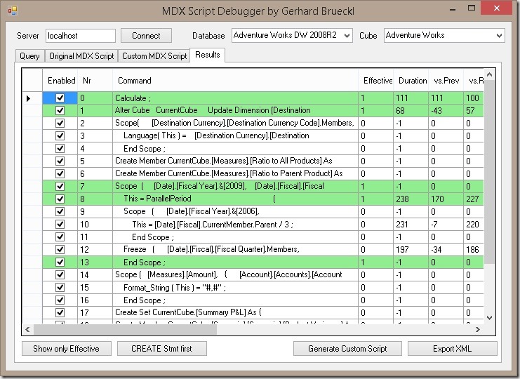
I recently built a tool which should help to debug the MDX scripts of an Analysis Services cube in order to track down formula engine related performance issues of a cube. As you probably know most of the performance issues out there are usually caused by poorly or wrong written MDX scripts. This tool allows you to execute a reference query and highlights the MDX script commands that are effectively used when the query is run. It provides the overall timings and how long each additional MDX script command extended the execution time of the reference query. The results can then either be exported to XML for further analysis in e.g. Power BI or a customized version of the MDX script can be created and used to run another set of tests.

The tool is currently in a beta state and this is the first official release – and also my first written tool that I share publicly so please don’t be too severe with your feedback Open-mouthed smile  – just joking every feedback is good feedback!

Below is a little screenshot which shows the results after  the reference query is executed. The green lines are effectively used by the query whereas the others do not have any impact on the values returned by the query.

ResultsView

A list of all features, further information and also the source code can be found at the project page on codeplex:
https://mdxscriptdebugger.codeplex.com/
Also the download is available from there:
https://mdxscriptdebugger.codeplex.com/releases

Looking forward to your feedback and hope it helps you to track down performance issues of your MDX Scripts!

Reporting Services MDX Field List and Using Measures on rows

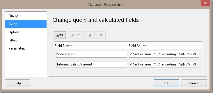
When creating a Reporting Services report on top of an Analysis Services cube using the wizard it automatically creates a Field for each column in your MDX query. Those fields can then be used in your report. For reports based on a relational source the definition of these fields is quite simple, it is the same as the the column name of the originating query. For MDX queries this is very different. If you ever checked the definition of an automatically generated MDX field you will see a lengthy XML snippet instead:
FieldsList

The XMLs may look like these:

<?xml version="1.0" encoding="utf-8"?>
<Field xmlns:xsi="http://www.w3.org/2001/XMLSchema-instance"
       xmlns:xsd="http://www.w3.org/2001/XMLSchema"
       xsi:type="Level"
       UniqueName="[Product].[Subcategory].[Subcategory]" />

<?xml version="1.0" encoding="utf-8"?>
<Field xmlns:xsi="http://www.w3.org/2001/XMLSchema-instance"
       xmlns:xsd="http://www.w3.org/2001/XMLSchema"
       xsi:type="Measure"
       UniqueName="[Measures].[Internet Sales Amount]" />

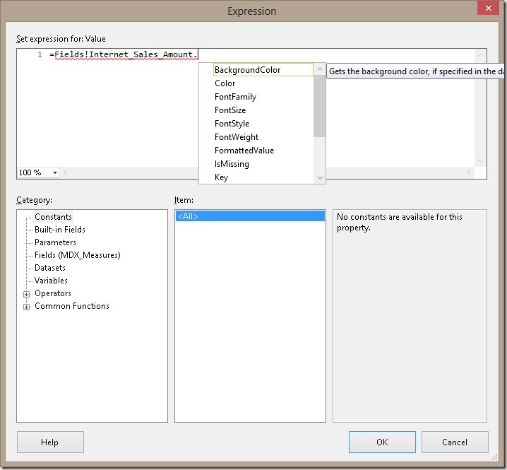
As you can see those two are quite different in terms of xsi:type and UniqueName. The xsi:type “Level” refers to a dimension level whereas “Measure” refers to a measure. Depending on the type of field, different properties are available within the report:
FieldProperties

For example the property BackgroundColor is only populated for fields of type “Measure” whereas the property UniqueName is only populated for fields of type “Level”. Measure properties are tied to the CELL PROPERTIES in your MDX query and Level properties are tied to DIMENSION PROPERTIES:

SELECT
NON EMPTY { [Measures].[Internet Sales Amount] } ON COLUMNS,
NON EMPTY { ([Product].[Subcategory].[Subcategory].ALLMEMBERS ) }
DIMENSION PROPERTIES MEMBER_CAPTION, MEMBER_UNIQUE_NAME ON ROWS
FROM [Adventure Works]
CELL PROPERTIES VALUE, BACK_COLOR, FORE_COLOR, FORMATTED_VALUE, FORMAT_STRING, FONT_NAME, FONT_SIZE, FONT_FLAGS

If we remove MEMBER_UNIQUE_NAME from the DIMENSION PROPERTIES we would no longer be able to use Fields!Subcategory.UniqueName in our SSRS expressions, or to be more precise it would simply always return NULL (or NOTHING in terms of Visual Basic). The same of course is also true for the CELL PROPERTIES.

So far this is nothing really new but there are some more things about the fields of MDX queries. There is a third xsi:type called “MemberProperty” which allows you to query member properties without having to define separate measures within your query:

<?xml version="1.0" encoding="utf-8"?>
<Field xmlns:xsi="http://www.w3.org/2001/XMLSchema-instance"
       xmlns:xsd="http://www.w3.org/2001/XMLSchema"
       xsi:type="MemberProperty"
       LevelUniqueName="[Product].[Subcategory].[Subcategory]"
       PropertyName="Category" />

Once we add a member property to our MDX query SSRS also automatically creates this field for us. NOTE, this is only possible by manually modifying the MDX!

SELECT
NON EMPTY { [Measures].[Internet Sales Amount] } ON COLUMNS,
NON EMPTY { ([Product].[Subcategory].[Subcategory].ALLMEMBERS ) }
DIMENSION PROPERTIES MEMBER_CAPTION, MEMBER_UNIQUE_NAME,
    [Product].[Subcategory].[Subcategory].[Category] ON ROWS
FROM [Adventure Works]
CELL PROPERTIES VALUE, BACK_COLOR, FORE_COLOR, FORMATTED_VALUE, FORMAT_STRING, FONT_NAME, FONT_SIZE, FONT_FLAGS

To get the [Category] which is associated to a given [Subcategory] you would usually need to create a separate measure like this:

WITH
MEMBER [Measures].[Category] AS (
[Product].[Subcategory].Properties( "Category" )
)
SELECT

This has the very bad drawback that using the WITH MEMBER clause disables the formula engine cache for the whole query what may result in worse query performance. So you may consider using DIMENSION PROPERTIES instead of a custom Measure next time.


There is another very nice “feature” that is also related to the field list. If you ever had the requirement to create a parameter to allow the user to select which measure he wants to see in the report you probably came across this blog post by Chris Webb or this blog post by Rob Kerr. As you know by then, SSRS requires you to put the Measures-dimension on columns, otherwise the query is not valid. This is because the number of Measures is not considered to be dynamic (opposed to e.g. Customers) which allows SSRS to create a static field list. This makes sense as SSRS was originally designed for relational reporting and a table always has a fixed number of columns which are similar to fields in the final SSRS dataset. Using Measures on columns is the way how SSRS enforces this.

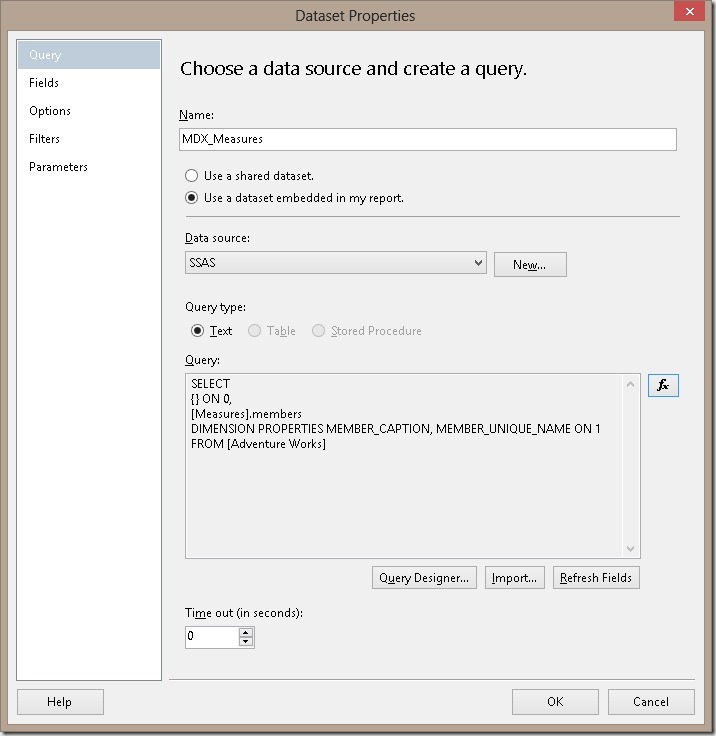
As we are all smart SSRS and MDX developers and we know what we are doing we can trick SSRS here. All we need to do is to write a custom MDX query using the expression builder – do not use or even open the Query Designer at this point otherwise your query may get overwritten!
Query_Measures

SSRS also automatically creates the fields for us, but this time the fields are not defined correctly. It creates one field with a very cryptic name and the following XML definition:

<?xml version="1.0" encoding="utf-8"?>
<Field xmlns:xsi="http://www.w3.org/2001/XMLSchema-instance"
       xmlns:xsd="http://www.w3.org/2001/XMLSchema"
       xsi:type="Measure"
       UniqueName="[Measures].[MeasuresLevel]" />

As you can see SSRS thinks that this field is of type “Measure” but it actually is a “Level”. After changing this little thing we can access all field properties that are unique to Level-fields like <Field>.UniqueName

So this is the final MDX query and the associated XML field definition:

SELECT
{} ON 0,
[Measures].members
DIMENSION PROPERTIES MEMBER_CAPTION, MEMBER_UNIQUE_NAME ON 1
FROM [Adventure Works]

Ensure that you have defined the necessary DIMENSION PROPERTIES here otherwise they will not be available/populated within the report!

<?xml version="1.0" encoding="utf-8"?>
<Field xmlns:xsi="http://www.w3.org/2001/XMLSchema-instance"
       xmlns:xsd="http://www.w3.org/2001/XMLSchema"
       xsi:type="Level"
       UniqueName="[Measures].[MeasuresLevel]" />

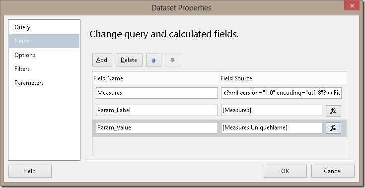
In order to make use of this approach in a report parameter we further need to create calculated fields for our parameter label and parameter value:
Fields_Measures
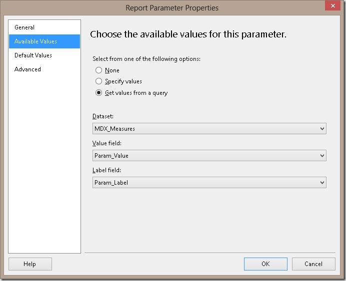
The definition of the parameter is straight forward then:
ParameterDefinition

You can not only use this approach to populate a parameter but you can also use it to crossjoin Measures on rows with any other hierarchy. This way you can avoid writing complex MDX just to work around this nasty SSRS limitation.

Downloads:

Sample SSRS report: CustomFieldList.rdl

DAX vs. MDX: DataMembers in Parent-Child Hierarchies

Recently when browsing the MSDN PowerPivot Forums I came across this thread where the question was ask on how to show the value which is directly linked to an element in a parent-child hierarchy instead of the aggregation of all "children". In this post I am going to address this problem finally showing a proper solution.


First of all I would like to start with some background to so called "datamembers". The term "datamember" originates from parent-child hierarchies in multidimensional models. It is a dummy-member that is created automatically below each hierarchy-node to hold values that are linked to a node-member directly. This is of course only possible for parent-child hierarchies.

Take the following MDX-Query for example:

SELECT
[Measures].[Sales Amount Quota] ON 0,
Descendants(
    [Employee].[Employees].&[290],
    1,
    SELF_AND_BEFORE) ON 1
FROM [Adventure Works]
WHERE [Date].[Calendar].[Calendar Year].&[2006]

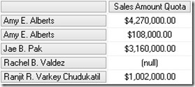
HiddenDatamember

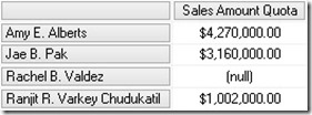
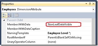
As we can see, the value of "Amy E. Alberts" is not the Sum of its children but has a difference of $108,000.00 This difference is because of the "datamember" that is also a child of every parent-child node which may be hidden. For multidimensional models his behavior can be changed by setting the MembersWithData-Property to "NonLeafDataVisible":

VSProperties


Executing the same query again we now get this results:

VisibleDatamember

Now we see "Amy E. Alberts" twice – the node and the datamember.


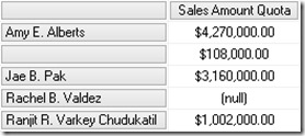
Doing a similar query on a tabular model we will get this result by default:

q4evw0ne

As you can see, we still have the datamember but without any caption. Though, this can of course be changed when you flatten out the hierarchy using DAX by simply replacing BLANK() by "<my datamember caption>" in your calculated columns.


Anyway, this is not the topic of this post but just some background information. Now we will focus on how to query data that is directly associated to a node or its corresponding datamember in MDX and DAX.


MDX:

For MDX this is quite easy as the datamember can be referenced by simply using ".datamember" of a given hierarchy node:

WITH

MEMBER [Measures].[DataMember] AS (
[Measures].[Sales Amount Quota],
[Employee].[Employees].currentmember.datamember
), FORMAT_STRING = 'Currency'

SELECT
{
[Measures].[Sales Amount Quota],
[Measures].[DataMember]
} ON 0,
Descendants(
    [Employee].[Employees].&[290],
    1,
    SELF_AND_BEFORE) ON 1
FROM [Adventure Works]
WHERE [Date].[Calendar].[Calendar Year].&[2006]

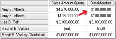
DatamemberValue_MDX

The DataMember-Measure only shows values that are directly linked to the current node of the parent-child hierarchy. This is pretty straight forward and very easy to accomplish.


DAX:

In this DAX this problem is a bit more tricky as we do not have that built-in ".datamember" function. Also navigation within hierarchies and parent-child hierarchies itself are not really supported in DAX. Though, there are several blogs out there that describe how to handle parent-child hierarchies by Alberto Ferrari (here) and Kasper de Jonge (here). Based on these solutions we can create our datamember-calculation.

First (and only) thing we need is to add a calculated column that stores the path depth of the current row. This can be achieved by using this formula:

=PATHLENGTH(
    PATH(
        Employee[EmployeeKey],
        Employee[ParentEmployeeKey]
    )
)


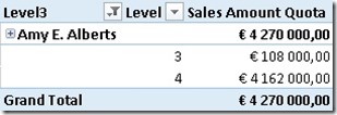
Using our previous example and selecting "Amy E. Alberts" together with our new column we get this:

CalculatedColumn_Level

As we can see there are two different Levels below "Amy E. Alberts" where Level=3 holds our datamember-value and Level=4 holds all the other values (=real child members). Lets add a calculated measure to help you make the final calculation more understandable:

MinLevel:=MIN(Employee[Level])

Calculation_MinLevel

So, for our [DataMember]-calculation we simply have to extend the context to only include rows where [Level] = [MinLevel]

DataMember:=CALCULATE(
SUM('Sales Quota'[Sales Amount Quota]),
FILTER('Employee',
    'Employee'[Level] = [MinLevel]))

CalculationNotWorking_DAX

Well, obviously our calculation is not returning the expected results. This is because of a very common pitfall which I am also very prone to. Whenever a calculated measure is used within an other calculated measure, a CALCULATE() gets wrapped around it thereby taking over the current context. In our case this means that ‘Employee'[Level] will always be the same as [MinLevel] as [MinLevel] gets evaluated for each row and doing MIN() on only one row of course always returns the value of the current row which we compared it to!

To solve this issue we have to place the original [MinLevel]-calculation directly into our [DataMember]-calculation:

DataMember:=CALCULATE(
SUM('Sales Quota'[Sales Amount Quota]),
FILTER('Employee',
    'Employee'[Level] = MIN(Employee[Level])))

CalculationWorking_DAX

This change finally makes the calculation return the correct results also when browsing using the hierarchy:

DatamemberValue_DAX


Even though DAX is not very good in handling hierarchies, the [DataMember]-calculation can be accomplished quite easily. This calculation also works for hierarchies of any depth without needing to adopt it. In terms of performance it may be further improved to the following formula – though the impact will be minor:

DataMember_v2:=CALCULATE(
SUM('Sales Quota'[Sales Amount Quota]),
FILTER(VALUES('Employee'[Level]),
    'Employee'[Level] = MIN(Employee[Level])))


Download Final Model (Office 2013!)

Another Post about Calculating New and Returning Customers – Part 2

In my previous post I showed a new approach on how to calculate new (and returning) customers in PowerPivot/tabular using DAX. We ended up with a solution where we added the customers first order date as a calculated column to our customer-table. This column was then linked to our date-table with an inactive relationship. The final calculation used USERELATIONSHIP() to make use of this relationship as follows:

New Customers:=CALCULATE(
COUNTROWS(Customer),
USERELATIONSHIP(Customer[FirstOrderDate], ‘Date’[Date]))

This calculation performs really well as it does not have to touch the fact-table to get the count of new customers. And this is also the issue with the calculation as other filters are not reflected in the calculation:

Issue_Old_vs_New

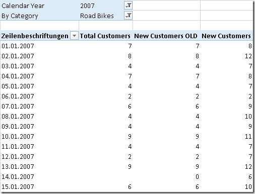
Take row 2 as an example: we have 8 “Total Customers” of which 12 are “New Customers”. Obviously an error in the calculation. The PivotTable is filtered to Category=”Road Bikes” and we have 8 customers on the 2nd of February that bought a road bike. The “New Customers” calculation on the other hand is not related to the Subcategory and shows 12 as in total there were 12 new customers for all products.


To get our calculation working also with other filters we have to somehow relate it to our fact-table. So far we calculated the customers first order date only in the customer table. The customers first order may be related to several fact-rows, e.g. one row for each product the customer bought. Our “New Customers” calculation should only include customers that are active considering also all other filters.

To identify a customers first order in our fact-table we can again use a calculated column and also re-use our previous calculated column in our Customer-table that holds the customers first order date:

=NOT(
ISBLANK(
LOOKUPVALUE(
Customer[CustomerKey],
[CustomerKey],
Customer[FirstOrderDate],
[Order Date]
)))

This returns True for all fact-rows associated with a customers first order and False for all other rows.

The final “New Customers v2” calculation is quite simple then – in addition to the active filters we add a further filter to only select rows that are associated to a customers first order:

New Customers v2:=CALCULATE(
[Total Customers],
‘Internet Sales’[IsCustomersFirstOrder] = TRUE())


And this are the results:

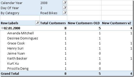
Final_Old_vs_NewV2

As you can see there are still differences between “New Customers OLD” and “New Customers v2”. But is this really a problem with the new calculation? Lets analyze the issue taking customer “Desiree Dominguez” where we encounter the first difference as an example:

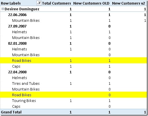
Issue_Analyzed

“Desiree Dominguez” had her first order on the 22th of June in 2006. So she is actually no “new customer” in 2008. The reason why the old calculation counts her as “new customer” is that it was the first time that she bought a product of subcategory “Road Bikes”. Whether this is correct or not is up to your business definition of a “new customer”. According to my experience it is more likely that “Desiree Dominguez” is not counted as a new customer in 2008 and so the “New Customer v2” actually returns the more accurate results.


Additional stuff:

An other option for this calculation is to rank the [Order Date] or [Sales Order Number] for each customer within the fact-table using the calculation below:

=RANKX(
FILTER(
ALL(‘Internet Sales’),
[CustomerKey] = EARLIER([CustomerKey])),
[Order Date],
[Order Date],
1,
DENSE
)

[Order Date] could be replaced by [Sales Order Number]. This makes sense if a customer can have multiple orders per day and you also want to distinguish further by [Sales Order Number]. The new field would also allow new analysis. For example the increase/decrease in sales from the second order compared to the first order and so on.

The “New Customer” calculation in this case would still be similar. We just have to filter on the new calculated column instead:

New Customers v3:=CALCULATE(
[Total Customers],
‘Internet Sales’[CustomersOrderNr] = 1)


Download Final Model (Office 2013!)


The multidimensional model:

The whole logic of extending the fact-table to identify rows that can be associated with a customers first order can also be used in a multidimensional model. Once we prepared the fact-table accordingly the calculations are quite easy. The biggest issues here does not reside in the multidimensional model itself but in the ETL/relational layer as this kind of operation can be quite complex – or better say time-consuming in terms of ETL time.

At this point I will not focus on the necessary ETL steps but start with an already prepared fact-table and highlight the extensions that have to be made in the multidimensional model. The fact-table already got extended by a new column called [IsCustomersFirstOrder] similar to the one we created in tabular using a DAX calculated column. It has a value of 1 for rows associated with a customers first order and 0 for all other rows.

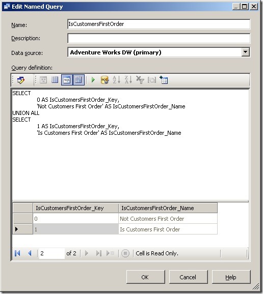
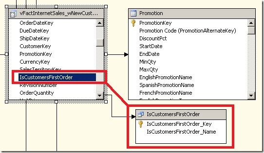
The next thing we have to do is to create a new table in our DSV to base our new dimension on. For simplicity I used this named query:

MD_NamedQuery_Dim

This table is then joined to the new fact-table:

MD_DSV

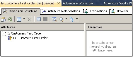
The new dimension is quite simple as it only contains one attribute:

MD_Dimension

You may hide the whole dimension in the end as it may only be used to calculate our “new customers” and nowhere else and may only confuse the end-user.


Once we have added the dimension also to our cube we can create a new calculated measure to calculate our “new customers” as follows:

CREATE MEMBER CURRENTCUBE.[Measures].[New Customers] AS (
[Measures].[Customer Count],
[Is Customers First Order].[Is Customers First Order].&[1]
), ASSOCIATED_MEASURE_GROUP = ‘Internet Customers’
, FORMAT_STRING = ‘#,##0’;

The calculation is based on the existing [Customer Count]-measure which uses DistinctCount-aggregation. Similar to DAX with just extend the calculation by further limiting the cube-space where “Is customers First Order” = 1.

This approach also allows you to create aggregations if necessary to further improve performance. So this is probably also the best way in terms of query-performance to calculate the count of new customers in a multidimensional model.