A very common requirement in reporting is to show the Top N items (products, regions, customers, …) and this can also be achieved in Power BI quite easily.
But lets start from the beginning and show how this requirement usually evolves and how to solve the different stages.
The easiest thing to do is to simply resize the visual (e.g. table visual) to only who 5 rows and sort them descending by your measure:
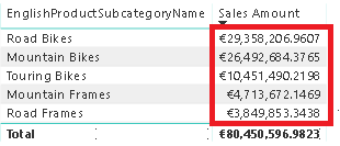
This is very straight forward and I do not think it needs any further explanation.
The next requirement that usually comes up next is that the customer wants to control, how many Top items to show. So they implement a slicer and make the whole calculation dynamic as described here:
SQL BI – Use of RANKX in a Power BI measure
FourMoo – Dynamic TopN made easy with What-If Parameter
Again, this works pretty well and is explained in detail in the blog posts.
Once you have implemented this change the business users usually complain that Total is wrong. This depends on how you implemented the TopN measure and what the users actually expect. I have seen two scenarios that cause confusion:
1) The Total is the SUM of the TopN items only – not reflecting the actual Grand Total
2) The Total is NOT the SUM of the TopN items only – people complaining that Power BI does not sum up correctly
As I said, this pretty much depends on the business requirements and after discussing that in length with the users, the solution is usually to simply add an “Others” row that sums up all values which are not part of the TopN items. For regular business users this requirement sounds really trivial because in Excel the could just add a new row and subtract the values of the TopN items from the Grand Total.
However, they usually will not understand the complexity behind this requirement for Power BI. In Power BI we cannot simply add a new “Others” row on the fly. It has to be part of the data model and as the TopN calculations is already dynamic, also the calculation for “Others” has to be dynamic. As you probably expected, also this has been covered already:
Oraylis – Show TopN and rest in Power BI
Power BI community – Dynamic Top N and Others category
These work fine even if I do not like the DAX as it is unnecessarily complex (from my point of view) but the general approach is the same as the one that will I show in this blog post and follows these steps:
1) create a new table in the data model (either with Power Query or DAX) that contains all our items that we want to use in our TopN calculation and an additional row for “Others”
2) link the new table also to the fact table, similar to the original table that contains your items
3) write a measure that calculates the rank for each item, filters the TopN items and assigns the rest to the “Others” item
4) use the new measure in combination with the new table/column in your visual
Step 1 – Create table with “Others” row
I used a DAX calculated table that does a UNION() of the existing rows for the TopN calculation and a static row for “Others”. I used ROW() first so I can specify the new column names directly. I further use ALLNOBLANKROW() to remove to get rid of any blank rows.
Subcategory_wOthers = UNION(
ROW("SubcategoryKey_wOthers", -99, "SubcategoryName_wOthers", "Others"),
ALLNOBLANKROW('ProductSubcategory'[ProductSubcategoryKey], 'ProductSubcategory'[SubcategoryName])
)
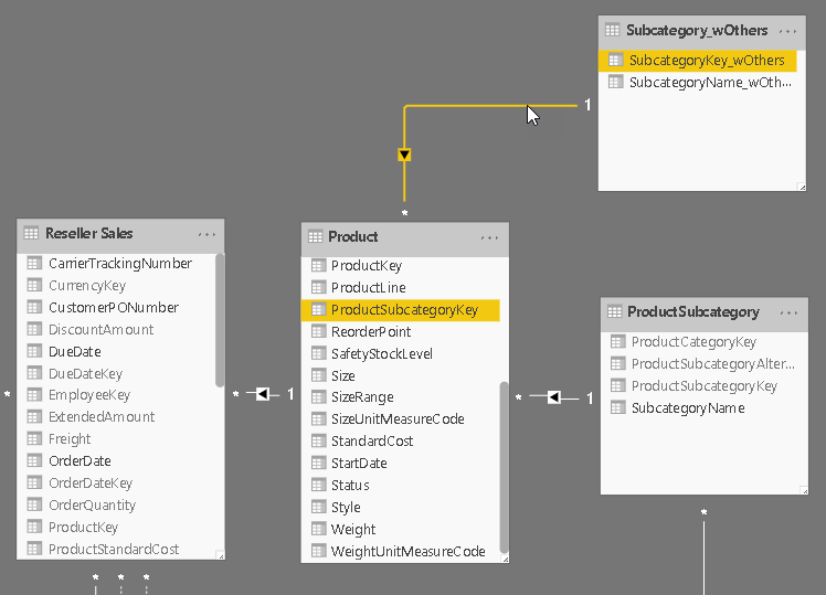
Step 2 – Create Relationship
The new table is linked to the same table to which the original table was linked to. This can be the fact-table directly or an intermediate table that then filters the facts in a second step (as shown below)
Step 3 – Create DAX measure
That’s actually the tricky part about this solution, but I think the code is still very easy to read and understand:
Top Measure ProductSubCategory =
/* get the items for which we want to calculate TopN + Others */
VAR Items = SELECTCOLUMNS(ALL(Subcategory_wOthers), "RankItem", Subcategory_wOthers[SubcategoryName_wOthers])
/* add a measure that we use for ranking */
VAR ItemsWithValue = ADDCOLUMNS(Items, "RankMeasure", CALCULATE([Selected Measure], ALL(ProductSubcategory)))
/* add a column with the rank of the measure within the items */
VAR ItemsWithRank = ADDCOLUMNS(ItemsWithValue, "Rank", RANKX(ItemsWithValue, [RankMeasure], [RankMeasure], DESC, Dense))
/* calculate whether the item is a Top-item or belongs to Others */
VAR ItemsWithTop = ADDCOLUMNS(ItemsWithRank, "TopOrOthers", IF([Rank] <= [Selected TopN], [RankItem], "Others"))
/* select the final items for which the value is calculated */
VAR ItemsFinal = SELECTCOLUMNS( /* we only select a single column to be used with TREATAS() in the final filter */
     FILTER(
         ItemsWithTop,
         CONTAINSROW(VALUES(Subcategory_wOthers[SubcategoryName_wOthers]), [TopOrOthers]) /* need to obey current filters on _wOthers table. e.g. after Drill-Down */
         && CONTAINSROW(VALUES(ProductSubcategory[SubcategoryName]), [RankItem])), /* need to obey current filters on base table */
     "TopN_Others", [RankItem])
RETURN
CALCULATE(
    [Selected Measure],
    TREATAS(ItemsFinal, Subcategory_wOthers[SubcategoryName_wOthers])
)
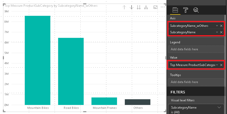
Step 4 – Build Visual
One of the benefits of this approach is that it also allows you to use the “Others” value in slicers, for cross-filtering/-highlight and even in drill-downs. To do so we need to configure our visual with two levels. The first one is the column that contains the “Others” item and the second level is the original column that contains the items. The DAX measure will take care of the rest.
And that’s it! You can now use the column that contains the artificial “Others” in combination with the new measure wherever you like. In a slicer, in a chart or in a table/matrix!
The final PBIX workbook can also be downloaded: TopN_Others.pbix


