Optimizing Columnar Storage for Measures

First of all I have to thank Marco Russo for his blog post on Optimizing High Cardinality Columns in Vertipaq and also his great session at SQL PASS Rally Nordic in Stockholm last year which taught me a lot about columnar storage in general. I highly recommend everyone to read the two mentioned resources before continuing here. Most of the ideas presented in this post are based on these concepts and require at least basic knowledge in columnar storage.

When writing one of my recent posts I ended up with a Power Pivot model with roughly 40M rows. It contained internet logs from Wikipedia, how often someone clicked on a given page per month and how many bytes got downloaded. As you can imagine those values can vary very heavily, especially the amount of bytes downloaded. So in the Power Pivot model we end up having a lot of distinct values in our column that we use for our measure. As you know from Marcos posts, the allocated memory and therefore also the  performance of columnar storage systems is directly related to the number of distinct values in a column – the more the worse. Marco already described an approach to split up a single column with a lot of distinct values into several columns with less distinct values to optimize storage. These concepts can also be used on columns that contain measures or numeric values in general. Splitting numeric values is quite easy, assuming your values range from 1 to 1,000,000 you can split this column into two by dividing the value by 1000 and using MOD 1000 for the second column. Instead of one column with the value 123,456 you end up with two columns with the values 123 and 456. In terms of storage this means that instead of 1,000,000 distinct values we only need to store 2 x 1,000 distinct values. Nothing new so far.

The trick is to combine those columns again at query time to get the original results as before the split. For some aggregations like SUM this is pretty straight forward, others are a bit more tricky. Though, in general the formulas are not really very complex and can be adopted very easily to handle any number of columns:

Aggregation DAX Formula
Value_SUM1 =SUMX(‘1M_Rows_splitted’, [Value_1000] * 1000 + [Value_1])
Value_SUM2 =SUM ( ‘1M_Rows_splitted'[Value_1000] ) * 1000
    + SUM ( ‘1M_Rows_splitted'[Value_1] )
Value_MAX =MAXX(‘1M_Rows_splitted’, [Value_1000] * 1000 + [Value_1])
Value_MIN =MINX(‘1M_Rows_splitted’, [Value_1000] * 1000 + [Value_1])
Value_COUNT =COUNTX(‘1M_Rows_splitted’, [Value_1000] * 1000 + [Value_1])
Value_DISTINCTCOUNT =COUNTROWS (
    SUMMARIZE (
        ‘1M_Rows_splitted’,
        ‘1M_Rows_splitted'[Value_1000],
        ‘1M_Rows_splitted'[Value_1]))

As you can see you can still mimic most kind of aggregation even if the [Value]-column is split up.

Though, don’t exaggerate splitting your columns – too many may be a bit inconvenient to handle and may neglect the effect resulting in worse performance. Marco already showed that you can get a reduction of up to 90% in size, during my simple tests I came up with about the same numbers. Though, it very much depends on the number of distinct values that you actually have in your column!

I would not recommend to always use this approach for all your measure column – no, definitely not! First check how many distinct values your data/measures contain and decide afterwards. For 1 million distinct values it is probably worth it, for 10,000 you may reconsider using this approach. Most important here is to test this pattern with your own data, data model and queries! Test it in terms of size and of course also in terms of performance. It may be faster to split up columns but it may also be slower and it may be also different for each query that you execute against the tabular model / Power Pivot. Again, test with your own data, data model and queries to get representative results! 

Here is a little test that you may run on your own to test this behavior. Simple create the following Power Query using M, load the result into Power Pivot and save the workbook. It basically creates a table with 1 million distinct values (0 to 999,999) and splits this column up into two. You can just copy the workbook, remove the last step “Remove Columns” and save it again to get the “original” workbook and Power Pivot model.

let
    List1 = List.Numbers(0, 1000000),

    TableFromList = Table.FromList(List1, Splitter.SplitByNothing(), null, null, ExtraValues.Error),
    RenamedColumns = Table.RenameColumns(TableFromList,{{"Column1", "Value"}}),
    ChangedType1 = Table.TransformColumnTypes(RenamedColumns,{{"Value", type number}}),
    InsertedCustom = Table.AddColumn(ChangedType1, "Value_1000", each Number.RoundDown([Value] / 1000)),
    InsertedCustom1 = Table.AddColumn(InsertedCustom, "Value_1", each Number.Mod([Value], 1000)),
    ChangedType = Table.TransformColumnTypes(InsertedCustom1,{{"Value_1000", type number}, {"Value_1", type number}}),
    RemovedColumns = Table.RemoveColumns(ChangedType,{"Value"})
in
    RemovedColumns

This is what I ended up with when you compare those two workbooks:

  # distinct values Final Size
single column 1,000,000 14.4 MB
two columns 2 x 1,000 1.4 MB

We also get a reduction in size of 90%! Though, this is a special scenario …
In the real world, taking my previous scenario with the Wikipedia data as an example, I ended up with a reduction to 50%, still very good though. But as you can see the reduction factor varies very much.

Downloads:

Sample workbook with Power Query: 1M_Rows_splitted.xlsx
Reporting Services MDX Field List and Using Measures on rows

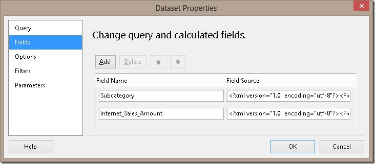
When creating a Reporting Services report on top of an Analysis Services cube using the wizard it automatically creates a Field for each column in your MDX query. Those fields can then be used in your report. For reports based on a relational source the definition of these fields is quite simple, it is the same as the the column name of the originating query. For MDX queries this is very different. If you ever checked the definition of an automatically generated MDX field you will see a lengthy XML snippet instead:
FieldsList

The XMLs may look like these:

<?xml version="1.0" encoding="utf-8"?>
<Field xmlns:xsi="http://www.w3.org/2001/XMLSchema-instance"
       xmlns:xsd="http://www.w3.org/2001/XMLSchema"
       xsi:type="Level"
       UniqueName="[Product].[Subcategory].[Subcategory]" />

<?xml version="1.0" encoding="utf-8"?>
<Field xmlns:xsi="http://www.w3.org/2001/XMLSchema-instance"
       xmlns:xsd="http://www.w3.org/2001/XMLSchema"
       xsi:type="Measure"
       UniqueName="[Measures].[Internet Sales Amount]" />

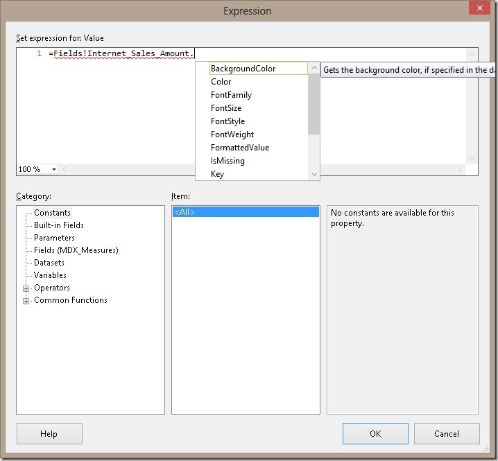
As you can see those two are quite different in terms of xsi:type and UniqueName. The xsi:type “Level” refers to a dimension level whereas “Measure” refers to a measure. Depending on the type of field, different properties are available within the report:
FieldProperties

For example the property BackgroundColor is only populated for fields of type “Measure” whereas the property UniqueName is only populated for fields of type “Level”. Measure properties are tied to the CELL PROPERTIES in your MDX query and Level properties are tied to DIMENSION PROPERTIES:

SELECT
NON EMPTY { [Measures].[Internet Sales Amount] } ON COLUMNS,
NON EMPTY { ([Product].[Subcategory].[Subcategory].ALLMEMBERS ) }
DIMENSION PROPERTIES MEMBER_CAPTION, MEMBER_UNIQUE_NAME ON ROWS
FROM [Adventure Works]
CELL PROPERTIES VALUE, BACK_COLOR, FORE_COLOR, FORMATTED_VALUE, FORMAT_STRING, FONT_NAME, FONT_SIZE, FONT_FLAGS

If we remove MEMBER_UNIQUE_NAME from the DIMENSION PROPERTIES we would no longer be able to use Fields!Subcategory.UniqueName in our SSRS expressions, or to be more precise it would simply always return NULL (or NOTHING in terms of Visual Basic). The same of course is also true for the CELL PROPERTIES.

So far this is nothing really new but there are some more things about the fields of MDX queries. There is a third xsi:type called “MemberProperty” which allows you to query member properties without having to define separate measures within your query:

<?xml version="1.0" encoding="utf-8"?>
<Field xmlns:xsi="http://www.w3.org/2001/XMLSchema-instance"
       xmlns:xsd="http://www.w3.org/2001/XMLSchema"
       xsi:type="MemberProperty"
       LevelUniqueName="[Product].[Subcategory].[Subcategory]"
       PropertyName="Category" />

Once we add a member property to our MDX query SSRS also automatically creates this field for us. NOTE, this is only possible by manually modifying the MDX!

SELECT
NON EMPTY { [Measures].[Internet Sales Amount] } ON COLUMNS,
NON EMPTY { ([Product].[Subcategory].[Subcategory].ALLMEMBERS ) }
DIMENSION PROPERTIES MEMBER_CAPTION, MEMBER_UNIQUE_NAME,
    [Product].[Subcategory].[Subcategory].[Category] ON ROWS
FROM [Adventure Works]
CELL PROPERTIES VALUE, BACK_COLOR, FORE_COLOR, FORMATTED_VALUE, FORMAT_STRING, FONT_NAME, FONT_SIZE, FONT_FLAGS

To get the [Category] which is associated to a given [Subcategory] you would usually need to create a separate measure like this:

WITH
MEMBER [Measures].[Category] AS (
[Product].[Subcategory].Properties( "Category" )
)
SELECT

This has the very bad drawback that using the WITH MEMBER clause disables the formula engine cache for the whole query what may result in worse query performance. So you may consider using DIMENSION PROPERTIES instead of a custom Measure next time.


There is another very nice “feature” that is also related to the field list. If you ever had the requirement to create a parameter to allow the user to select which measure he wants to see in the report you probably came across this blog post by Chris Webb or this blog post by Rob Kerr. As you know by then, SSRS requires you to put the Measures-dimension on columns, otherwise the query is not valid. This is because the number of Measures is not considered to be dynamic (opposed to e.g. Customers) which allows SSRS to create a static field list. This makes sense as SSRS was originally designed for relational reporting and a table always has a fixed number of columns which are similar to fields in the final SSRS dataset. Using Measures on columns is the way how SSRS enforces this.

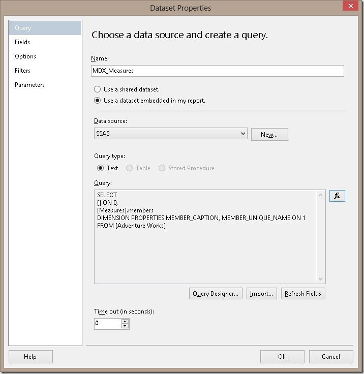
As we are all smart SSRS and MDX developers and we know what we are doing we can trick SSRS here. All we need to do is to write a custom MDX query using the expression builder – do not use or even open the Query Designer at this point otherwise your query may get overwritten!
Query_Measures

SSRS also automatically creates the fields for us, but this time the fields are not defined correctly. It creates one field with a very cryptic name and the following XML definition:

<?xml version="1.0" encoding="utf-8"?>
<Field xmlns:xsi="http://www.w3.org/2001/XMLSchema-instance"
       xmlns:xsd="http://www.w3.org/2001/XMLSchema"
       xsi:type="Measure"
       UniqueName="[Measures].[MeasuresLevel]" />

As you can see SSRS thinks that this field is of type “Measure” but it actually is a “Level”. After changing this little thing we can access all field properties that are unique to Level-fields like <Field>.UniqueName

So this is the final MDX query and the associated XML field definition:

SELECT
{} ON 0,
[Measures].members
DIMENSION PROPERTIES MEMBER_CAPTION, MEMBER_UNIQUE_NAME ON 1
FROM [Adventure Works]

Ensure that you have defined the necessary DIMENSION PROPERTIES here otherwise they will not be available/populated within the report!

<?xml version="1.0" encoding="utf-8"?>
<Field xmlns:xsi="http://www.w3.org/2001/XMLSchema-instance"
       xmlns:xsd="http://www.w3.org/2001/XMLSchema"
       xsi:type="Level"
       UniqueName="[Measures].[MeasuresLevel]" />

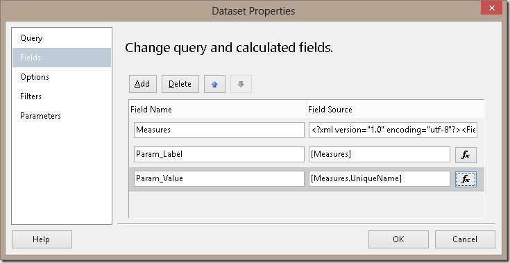
In order to make use of this approach in a report parameter we further need to create calculated fields for our parameter label and parameter value:
Fields_Measures
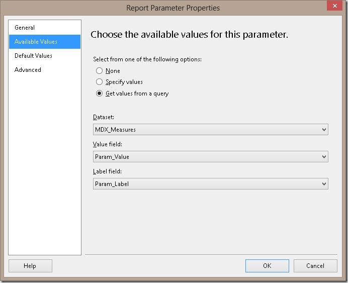
The definition of the parameter is straight forward then:
ParameterDefinition

You can not only use this approach to populate a parameter but you can also use it to crossjoin Measures on rows with any other hierarchy. This way you can avoid writing complex MDX just to work around this nasty SSRS limitation.

Downloads:

Sample SSRS report: CustomFieldList.rdl

Error-handling in Power Query

Data is the daily bread-and-butter for any analyst. In order to provide good results you also need good data. Sometimes this data is very well prepared beforehand and you can use it as it is but it is also very common that you need to prepare and transform the data on your own. To do this Microsoft has introduced Power Query (on tool of the Power BI suite). Power Query can be used to extract, transform and load data into Excel and/or Power Pivot directly.

When using any data you usually know what the data looks like and what to expect from certain columns – e.g. a value is delivered as a number, a text contains exactly 4 characters, etc.
Though, sometimes this does not apply for all rows of that dataset and your transformation logics may cause errors because of that. In order to avoid this and still have a clean data load you need to handle those errors. Power Query offers several options to this which I will elaborate in this post.

This is the sample data I will use for the following samples:

A B C
1 4 AXI23
2 5 TZ560
NA 6 UP945

we will perform simple transformations and type casts on this table to generate some errors:

Prepare_ChangeType

Error-handling on row-level

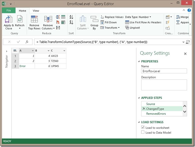
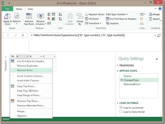
This is the easiest way of handling errors. Whenever a transformation causes an error, we can simply remove the whole row from the result set:

RowLevel_RemoveErrors

This will generate the following result table:

A B C
1 4 AX312
2 5 TZ560

As you can see, the third row was simply removed. This is the easiest way on how to remove errors from your result set but of course this may not be what you want as those removed rows may contain other important information in other columns! Assume you want to calculate the SUM over all values in column B. As we removed the third row we also removed a value from column B and the SUM is not the same as without the error-handling (9 vs. 15)!

Error-handling on cell-level

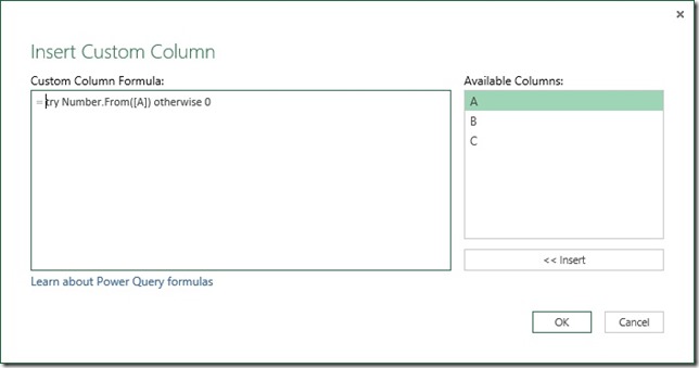
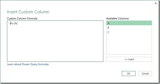
As we now know that column A may result in an error, we can handle this error during our transformation steps. As “NA” could not be converted to a number we see Error as result for that column. Clicking on it gives use some more details on the error itself. To handle this error we need to create a new calculated column where we first check if the value can be converted to a number and otherwise return a default numeric value:

RowLevel_RemoveErrors_CalcColumn

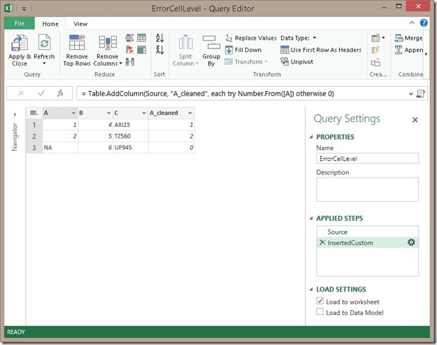
The M-function that we use is “try <expressions to try> otherwise <default if error>” which is very similar to a try-catch block in C#. If the expression causes an error, the default will be used instead. Details on the try-expression can be found in the Microsoft Power Query for Excel Formula Language Specification (PDF) which can be found here and is a must read for everyone interested in the M language.

CellLevel_HandleError

We could further replace our column A by the new column A_cleaned to hide this error handling transformation.

A B C A_cleaned
1 4 AXI23 1
2 5 TZ560 2
NA 6 UP945 0

Error-handling on cell-level with error details

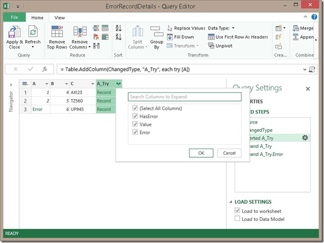
There may also be cases where it is OK to have one of this errors but you need/want to display the cause of the error so that a power user may correct the source data beforehand. Again we can use the try-function, but this time without the otherwise-clause. This will return a record-object for each row:

RowLevel_ShowErrors_CalcColumn

RowLevel_ShowErrors_Result1

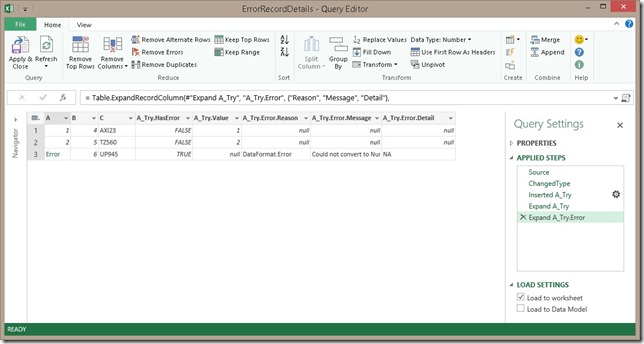
After expanding the A_Try column and also the A_Try.Error column we will get all available information on the error:

RowLevel_ShowErrors_Result2

A B C A_Try.HasError A_Try.Value A_Try.Error.Reason A_Try.Error.Message A_Try.Error.Detail
1 4 AXI23 FALSE 1
2 5 TZ560 FALSE 2
6 UP945 TRUE DataFormat.Error Could not convert to Number. NA

As you can see we get quite a lot of columns here. We could e.g. use A_Try.HasError to filter out error rows (similar to error-handling on row-level) or we could use it in a calculated column to mimic error-handling on cell-level. What you want to do with all the information is up to you, but in case you don’t need it you should remove all unnecessary columns.

Downloads:

Power Query Error Handling Workbook: Power Query Error Handling.xlsx
Trigger Cube-Processing from Excel using Cube Actions

Recently I faced the requirement to give specific users of my Analysis Services Multidimensional cube the opportunity to process the cube whenever they want. There are several ways to achieve this:
– start a SQL Agent that processes the cube
– create some kind of WebService that does the processing
– create some custom .NET application that does the processing
– run some script (PowerShell, Command Line, ascmd.exe, …)


NOTE:
The post describes a solution which requires SSAS Server Admin rights. If you are interested in a solution which triggers an asynchronous processing without requiring SSAS Server Admin Rights please scroll down to the very bottom and download VS_Solution.zip
It basically runs the same script but in a separate thread in the context of the service account so the calling user does not need to have any specific rights on the server.


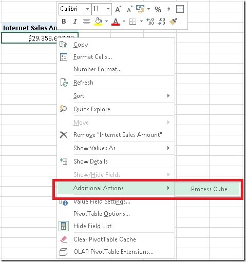
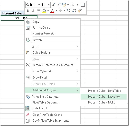
From a usability point-of-view none of the above is really convenient as all options involve some kind of external process or application. In this post I will show how to process a cube using cube actions which can be triggered from Excel Pivot Tables natively. So this is what we want to achieve:

Excel_Action


This requires several steps:
1) create custom .Net assembly
2) add that custom .Net assembly to your Analysis Services database
3) add an action to your cube that calls the assembly


Creating a Custom .Net assembly:

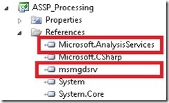
First of all we need to create a new “Visual C#” project of type “Class Library”. To work with Analysis Services we need to add two references:
VS_References

“Microsoft.AnalysisServices” refers to Microsoft.AnalysisServices.dll which  can be found in the shared features folder of your installation (default is c:Program FilesMicrosoft SQL Server110SDKAssemblies)

“msmgdsrv” refers to msmgdsrv.dll which can found be in the OLAPbin-folder of your SSAS instance (default is c:Program FilesMicrosoft SQL ServerMSAS11.MSSQLSERVEROLAPbin)

Once these references are added, we can start to create our processing code:

using System;
using AdomdServer = Microsoft.AnalysisServices.AdomdServer;
using Microsoft.AnalysisServices;
using System.Data;

namespace ASSP_Processing
{
    public class Processing
    {
        public const string LoggingPrefix = “ASSP.ProcessObject: “;
        public enum ResultHandling
        {
            Datatable = 0,
            Exception = 1,
            NULL = 2
        }

        public static DataTable ProcessObject(string cubeName, ResultHandling resultHandling)
        {
            DataTable ret = new DataTable();
            ret.Columns.Add(“Result”);

            Server server = null;

            try
            {
                server = new Server();

                //connect to the current session…
                server.Connect(“*”);

                AdomdServer.Context.CheckCancelled(); //could be a bit long running, so allow user to cancel

                Database db = server.Databases.GetByName(AdomdServer.Context.CurrentDatabaseName);

                string objectToProcessName = “#N/A”;
                ProcessableMajorObject objectToProcess = db;

                AdomdServer.Context.TraceEvent(0, 0, LoggingPrefix + “Database <“ + db.Name + “> found!”);
                objectToProcessName = “DB[“ + db.Name + “]”;

                if (!string.IsNullOrEmpty(cubeName))
                {
                    Cube cube = db.Cubes.GetByName(cubeName);

                    if (cube != null)
                    {
                        objectToProcess = cube;
                        AdomdServer.Context.TraceEvent(0, 0, LoggingPrefix + “Cube <“ + cubeName + “> found!”);
                        objectToProcessName = objectToProcessName + ” > Cube[“ + cubeName + “]”;
                    }
                }

                if (objectToProcess != null)
                {
                    AdomdServer.Context.TraceEvent(0, 0, LoggingPrefix + “Processing Object “ + objectToProcessName + ” …”);

                    objectToProcess.Process(ProcessType.ProcessFull);

                    ret.Rows.Add(new object[] { “S U C C E S S:    Object “ + objectToProcessName + ” successfully processed!” });
                    AdomdServer.Context.TraceEvent(0, 0, LoggingPrefix + “Finished Processing Object “ + objectToProcessName + “!”);
                }
            }
            finally
            {
                try
                {
                    if (server != null)
                        server.Disconnect();
                }
                catch { }
            }

            // if processing was successful a row has been added beforehand
            if (ret.Rows.Count == 0)
            {
                ret.Rows.Add(new object[] { “F A I L U R E:    Error while processing an object!” });
            }

            switch (resultHandling)
            {
                case ResultHandling.Datatable:
                    return ret;

                case ResultHandling.Exception:
                    throw new Exception(Environment.NewLine + Environment.NewLine + Environment.NewLine + ret.Rows[0][0].ToString());

                case ResultHandling.NULL:
                    return null;
            }

            return null;
        }

        public static DataTable ProcessObject(string cubeName, int resultHandling)
        {
            return ProcessObject(cubeName, (ResultHandling)resultHandling);
        }

        public static DataTable ProcessObject(string cubeName)
        {
            return ProcessObject(cubeName, 1);
        }
    }
}

There are two things here that are worth to point out. First of all we need to somehow establish a connection to the server that hosts the SSAS database in order to process an object. The first thing that comes into mind would be to create a new connection to the server and run some processing XMLA. Unfortunately this does not work here because as this would result in a deadlock. The assembly will be called as a Rowset-Action which in terms of locking is similar to a query. So if we run separate processing command within our Rowset-Action this processing command can never be committed as there is always a query running on the database. The query (=Rowset-Action) will wait until the function is finished and the function waits until the processing is committed resulting in a classical deadlock!

To avoid this we need to connect to the current users sessions using “*” as our connection string:

//connect to the current session…
server.Connect(“*”);


The second thing to point out is the return value of our function. In order to be used in a Rowset-action, the function has to return a DataTable object. The results would then be displayed similar to a drill through and a separate worksheet would pop up in Excel showing the result:

Result_DataTable

From my point-of-view this can be a bit annoying as after each processing this new worksheet pops up and you loose the focus of the pivot table. So I investigated a bit and found another way to display the output of the processing.

When a drill through / action throws an exception, this will also be displayed in Excel without actually displaying the result of the drill through / action in a separate worksheet. By default it may look like this message:

Result_NULL

Well, not really much information here right?

To display more information, e.g. that the processing was successful (or not) we can throw our own exception in the code after processing is done:

Result_Exception

I added a separate parameter to control this behavior, in the code above the default would be option 3 – custom Exception.


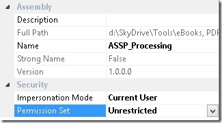
Once this project is built the DLL can be added to the SSAS database. It is necessary to grant the assembly “Unrestricted” permission set:

AssemblySettings


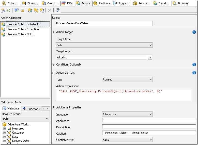
The last step would be to create the appropriate cube actions that call the assembly:

CubeActionConfiguration

It is necessary that the action is of Type=Rowset, otherwise it would not be displayed in Excel! The Action Target is up the you, in this example it will be displayed on every cell. The Action expression is the actual call to our assembly passing the cube name as a parameter. The second parameter controls how the result is displayed and could also be omitted.  In this example I added 3 separate actions, one for each result-type (as described above).

And that’s it! This simple steps allow you and your users to process any cube (or any other database object) from within your favorite client application, assuming it supports cube actions.

This is the final result where the three cube actions can be triggered from an Excel pivot table:

Excel_Action_Final


The attached zip-file includes everything that is necessary to recreate this example:
– SSAS project
– ASSP_Processing project

CubeProcessingAction.zip

Solution for Asynchronous Processing without Admin-Rights:
VS_Solution.zip

SSAS Dynamic Security and Visual Totals

Security is always an important aspect of any BI solution. Especially for big enterprise solutions the security-concept can become very complex. Analysis Services Multidimensional  in general offers two option on how to define security: Cell Data Permissions and Dimension Data Permissions. Because of the huge impact on performance Cell Data Permissions are barely used. Dimension Data Permissions are usually the way to go and can cover probably 98% of the security requirements. Though, also Dimension Data Permissions can get quite complex, especially for large-scale cubes with 100+ or even 1000+ users. Just think of an Analysis Services that holds sales data associated to KeyAccounts – further assume that we have 100 KeyAccounts. Each of this KeyAccounts is managed by one user, so we would end up creating 100 roles – one for each KeyAccount and its manager. In terms of maintenance this can get quite complex and in the long run unmanageable.

To address this issue Analysis Services offers the concept of Dynamic Security. Dynamic Security is evaluated at runtime for each user and allows you to consolidate your roles. So for our example from above instead of having 100 different roles we would end up having one dynamic role serving all 100 users. Basically, when a user connects it queries internal data (within the cube using MDX) or external data (using Analysis Services Stored Procedure (ASSP)/Assemblies) to get the security settings for the current user. Especially in combination with ASSP this can be quite powerful as you can use any datasource that you can query using .Net-code to derive your security from.

To make a role "dynamic" you basically have two options:
1) Username() – returns the current users in format "MyDomainMyUser"
2) CustomData() – returns whatever was specified in the connectionstring’s CustomData-property

Both are native MDX-functions and can be used in an expression to build your Allowed Set, Denied Set or DefaultMember.

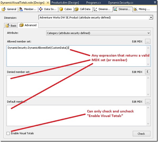
Role_UI

This works just fine, as long as the expressions returns a valid MDX set/member of course.
But what about the Visual Totals – setting? You can only check or uncheck the checkbox and you are not able to use any dynamic expressions. That’s what the UI offers you – no more no less. But there might be some rare scenarios where you also need to make the Visual Totals dynamically based on Username() or CustomData() – and this is what this post is about.


So, as we have already seen above, it is not possible to make the Visual Totals dynamically using the UI. Fortunately there are also other ways besides the UI to work with the cube and modify its structure. I am talking about XMLA (XML for Analysis Services) here, which is the protocol that is used for all communications between a client and Analysis Services. Instead of writing XMLA on your own there is also a programmatically way to do this: AMO (Analysis Management Object). AMO is a .Net library that allows you to integrate calls to Analysis Services within any .Net code. After modifying any object in the code AMO generates the according XMLA for you and sends it to the server which is a much more convenient way than writing plane XMLA on your own.

This means that you can also create/modify your security roles using AMO – this approach is already very well described by Benny Austin in his blog about SSAS: Using AMO to Secure Analysis Service Cube. I recommend reading this article before you continue here.

For this little example I create a slimmed down version of Adventure works. The model contains only the Date and the Product dimension. We will put our dynamic security on the Category attribute of our Product dimension. The model also already contains a predefined empty role called "DynamicVisualTotals" that we will modify later (after the model has been deployed) using AMO. Please note here that AMO only work with the Analysis Service directly (online) but not at design time in Visual Studio. Once everything is deployed this is the AMO code to use to modify the predefined role:

using Microsoft.AnalysisServices;

namespace ModifyRole_AMO
{
    class Program
    {
        static void Main(string[] args)
        {
            using (Server oServer = new Server())
            {
                oServer.Connect("localhost");

                using (Database oDB = oServer.Databases.GetByName("DynamicVisualTotals"))
                {
                    Role oRole = oDB.Roles.GetByName("DynamicVisualTotals");

                    Dimension oDim = oDB.Dimensions.GetByName("Product");
                    DimensionAttribute oAttr = oDim.Attributes.FindByName("Category");
                    DimensionPermission oDimPermission = oDim.DimensionPermissions.FindByRole(oRole.ID);

                    AttributePermission oAttrPermission = oDimPermission.AttributePermissions.Find(oAttr.ID);

                    // can be done in the UI
                    oAttrPermission.AllowedSet = "DynamicSecurity.DynamicAllowedSet(CustomData())";
                    // can not be done in the UI
                    oAttrPermission.VisualTotals = "DynamicSecurity.DynamicVisualTotals(CustomData())";

                    oDimPermission.Update();
                }
            }
        }
    }
}

1) connect to server "localhost"
2) connect to database "DynamicVisualTotals"
3) get the Role-object for role "DynamicVisualTotals" from the database
4) get the Dimension-object for dimension "Product"
5) get the DimensionAttribute-object for attribute "Category"
6) get the DimensionPermission that is associated to our Role for dimension "Product"
7) get the AttributePermission that is associated to our attribute "Category"

So far this is straight forward. The AttributePermission object actually represents the UI that we have seen above. It has properties for all the fields and textboxes on the UI. The most important of course are:
– AllowedSet
– DeniedSet
– Defaultmember
– and VisualTotals

For the first three I was already aware that they are of type String but the VisualTotals I expected to be Boolean which turned out to be wrong – it is also a String!

VisualTotalsIsString 

Naïve as I am I simply put a MDX expression in there that resolves to "1" or "0" (Boolean, similar to the Checkbox in the UI, it could probably also resolve to "true" or "false" or a Boolean type directly but I did not further test this) – and, it worked like a charm! The MDX expression I used refers to an ASSP called DynamicSecurity which contains a function called "DynamicVisualTotals" that returns "1" or "0" based on what was passed in the connectionstring using CustomData():

using Microsoft.AnalysisServices.AdomdServer;

namespace DynamicSecurity
{
    public static class DynamicSecurity
    {
        public static string DynamicVisualTotals(string customData)
        {
            if (customData == "1")
                return "1";

            return "0";
        }

        public static Set DynamicAllowedSet(string customData)
        {
            string mdxEpression;
            Expression exp;
            Set s;

            if (customData == "1")
                mdxEpression = "{[Product].[Category].&[1]}";

            else
                mdxEpression = "{[Product].[Category].&[3], [Product].[Category].&[4]}";

            exp = new Expression(mdxEpression);
            s = exp.CalculateMdxObject(null).ToSet();

            return s;
        }
    }
}

(This ASSP has to be compiled and added to the database first to make the Dynamic Security work. This is describe here in more detail.)

And that’s it!

Once everything is done
1) Deploy the solution to the sever
2) (add ASSP if not already included in the solution)
3) Execute the AMO code (first listing)
we can use Excel to check the results:

FinalResults


The used connection strings are as follows:

Provider=MSOLAP.5;Integrated Security=SSPI;Persist Security Info=True;Data Source=localhost;Initial Catalog=DynamicVisualTotals;Roles=DynamicVisualTotals;CustomData=0


Provider=MSOLAP.5;Integrated Security=SSPI;Persist Security Info=True;Data Source=localhost;Initial Catalog=DynamicVisualTotals;Roles=DynamicVisualTotals;CustomData=1

Make sure to also use the Roles-property for testing as if you are administrator these privileges would overwrite all other security settings!


Additional Notes:

As AMO is just a wrapper for XMLA we could also use XMLA directly to modify our role:

<Alter AllowCreate="true" ObjectExpansion="ObjectProperties" xmlns="http://schemas.microsoft.com/analysisservices/2003/engine">
    <Object>
        <DatabaseID>DynamicVisualTotals</DatabaseID>
        <DimensionID>Dim Product</DimensionID>
        <DimensionPermissionID>DimensionPermission</DimensionPermissionID>
    </Object>
    <ObjectDefinition>
        <DimensionPermission xmlns:xsd="http://www.w3.org/2001/XMLSchema" xmlns:xsi="http://www.w3.org/2001/XMLSchema-instance" xmlns:ddl2="http://schemas.microsoft.com/analysisservices/2003/engine/2" xmlns:ddl2_2="http://schemas.microsoft.com/analysisservices/2003/engine/2/2" xmlns:ddl100_100="http://schemas.microsoft.com/analysisservices/2008/engine/100/100" xmlns:ddl200="http://schemas.microsoft.com/analysisservices/2010/engine/200" xmlns:ddl200_200="http://schemas.microsoft.com/analysisservices/2010/engine/200/200" xmlns:ddl300="http://schemas.microsoft.com/analysisservices/2011/engine/300" xmlns:ddl300_300="http://schemas.microsoft.com/analysisservices/2011/engine/300/300" xmlns:ddl400="http://schemas.microsoft.com/analysisservices/2012/engine/400" xmlns:ddl400_400="http://schemas.microsoft.com/analysisservices/2012/engine/400/400">
            <ID>DimensionPermission</ID>
            <Name>DimensionPermission</Name>
            <RoleID>Role</RoleID>
            <Read>Allowed</Read>
            <AttributePermissions>
                <AttributePermission>
                    <AttributeID>Product Category Name</AttributeID>
                    <AllowedSet>DynamicSecurity.DynamicAllowedSet(CustomData())</AllowedSet>
                    <VisualTotals>DynamicSecurity.DynamicVisualTotals(CustomData())</VisualTotals>
                </AttributePermission>
            </AttributePermissions>
        </DimensionPermission>
    </ObjectDefinition>
</Alter>


Please note that XMLA always uses the internal IDs which may not be the same as the name of the objects!


In this post I showed how to use AMO and XMLA to modify a security role and use an expression to make the VisualTotals setting dynamic which is not possible using the UI only. This is just a very simplified example but I used this approach on some of my enterprise deployments and it works just fine also for very complex scenarios.


The attached zip-file includes everything that is necessary to recreate this example:
– SSAS project
– ASSP project
– AMO project (and XMLA script)
– final Excel with results

DynamicVisualTotals.zip

DAX vs. MDX: DataMembers in Parent-Child Hierarchies

Recently when browsing the MSDN PowerPivot Forums I came across this thread where the question was ask on how to show the value which is directly linked to an element in a parent-child hierarchy instead of the aggregation of all "children". In this post I am going to address this problem finally showing a proper solution.


First of all I would like to start with some background to so called "datamembers". The term "datamember" originates from parent-child hierarchies in multidimensional models. It is a dummy-member that is created automatically below each hierarchy-node to hold values that are linked to a node-member directly. This is of course only possible for parent-child hierarchies.

Take the following MDX-Query for example:

SELECT
[Measures].[Sales Amount Quota] ON 0,
Descendants(
    [Employee].[Employees].&[290],
    1,
    SELF_AND_BEFORE) ON 1
FROM [Adventure Works]
WHERE [Date].[Calendar].[Calendar Year].&[2006]

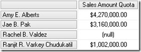
HiddenDatamember

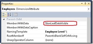
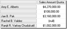
As we can see, the value of "Amy E. Alberts" is not the Sum of its children but has a difference of $108,000.00 This difference is because of the "datamember" that is also a child of every parent-child node which may be hidden. For multidimensional models his behavior can be changed by setting the MembersWithData-Property to "NonLeafDataVisible":

VSProperties


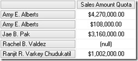
Executing the same query again we now get this results:

VisibleDatamember

Now we see "Amy E. Alberts" twice – the node and the datamember.


Doing a similar query on a tabular model we will get this result by default:

q4evw0ne

As you can see, we still have the datamember but without any caption. Though, this can of course be changed when you flatten out the hierarchy using DAX by simply replacing BLANK() by "<my datamember caption>" in your calculated columns.


Anyway, this is not the topic of this post but just some background information. Now we will focus on how to query data that is directly associated to a node or its corresponding datamember in MDX and DAX.


MDX:

For MDX this is quite easy as the datamember can be referenced by simply using ".datamember" of a given hierarchy node:

WITH

MEMBER [Measures].[DataMember] AS (
[Measures].[Sales Amount Quota],
[Employee].[Employees].currentmember.datamember
), FORMAT_STRING = 'Currency'

SELECT
{
[Measures].[Sales Amount Quota],
[Measures].[DataMember]
} ON 0,
Descendants(
    [Employee].[Employees].&[290],
    1,
    SELF_AND_BEFORE) ON 1
FROM [Adventure Works]
WHERE [Date].[Calendar].[Calendar Year].&[2006]

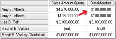
DatamemberValue_MDX

The DataMember-Measure only shows values that are directly linked to the current node of the parent-child hierarchy. This is pretty straight forward and very easy to accomplish.


DAX:

In this DAX this problem is a bit more tricky as we do not have that built-in ".datamember" function. Also navigation within hierarchies and parent-child hierarchies itself are not really supported in DAX. Though, there are several blogs out there that describe how to handle parent-child hierarchies by Alberto Ferrari (here) and Kasper de Jonge (here). Based on these solutions we can create our datamember-calculation.

First (and only) thing we need is to add a calculated column that stores the path depth of the current row. This can be achieved by using this formula:

=PATHLENGTH(
    PATH(
        Employee[EmployeeKey],
        Employee[ParentEmployeeKey]
    )
)


Using our previous example and selecting "Amy E. Alberts" together with our new column we get this:

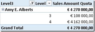
CalculatedColumn_Level

As we can see there are two different Levels below "Amy E. Alberts" where Level=3 holds our datamember-value and Level=4 holds all the other values (=real child members). Lets add a calculated measure to help you make the final calculation more understandable:

MinLevel:=MIN(Employee[Level])

Calculation_MinLevel

So, for our [DataMember]-calculation we simply have to extend the context to only include rows where [Level] = [MinLevel]

DataMember:=CALCULATE(
SUM('Sales Quota'[Sales Amount Quota]),
FILTER('Employee',
    'Employee'[Level] = [MinLevel]))

CalculationNotWorking_DAX

Well, obviously our calculation is not returning the expected results. This is because of a very common pitfall which I am also very prone to. Whenever a calculated measure is used within an other calculated measure, a CALCULATE() gets wrapped around it thereby taking over the current context. In our case this means that ‘Employee'[Level] will always be the same as [MinLevel] as [MinLevel] gets evaluated for each row and doing MIN() on only one row of course always returns the value of the current row which we compared it to!

To solve this issue we have to place the original [MinLevel]-calculation directly into our [DataMember]-calculation:

DataMember:=CALCULATE(
SUM('Sales Quota'[Sales Amount Quota]),
FILTER('Employee',
    'Employee'[Level] = MIN(Employee[Level])))

CalculationWorking_DAX

This change finally makes the calculation return the correct results also when browsing using the hierarchy:

DatamemberValue_DAX


Even though DAX is not very good in handling hierarchies, the [DataMember]-calculation can be accomplished quite easily. This calculation also works for hierarchies of any depth without needing to adopt it. In terms of performance it may be further improved to the following formula – though the impact will be minor:

DataMember_v2:=CALCULATE(
SUM('Sales Quota'[Sales Amount Quota]),
FILTER(VALUES('Employee'[Level]),
    'Employee'[Level] = MIN(Employee[Level])))


Download Final Model (Office 2013!)

Universal Quantiles Calculation for PowerPivot using DAX

In my last post I showed a new approach on how to calculate the median in PowerPivot using DAX. In the comments the question was raised whether it is possible to make that calculation universal for all kind of Quantiles like Median, Quartiles, Percentiles, etc. and that’s what this post is about.

Lets analyze the final Median calculation from the last post:

Median SA Months:=CALCULATE([SumSA],
TOPN(
2-MOD([Cnt_Months], 2),
TOPN(
([Cnt_Months] + 1) / 2,
VALUES(‘Date’[Month]),
[SumSA]),
[SumSA],
1))
/
(2-MOD([Cnt_Months], 2))


The Median defines the value in the middle of an ordered set. To get the first half (+1 to handle even and odd sets) of the whole we are using TOPN function:

TOPN(
([Cnt_Months] + 1) / 2,
VALUES(‘Date’[Month]),
[SumSA]),

The important part here is the “divide by 2” to split the set in the middle to start our Median calculation. Instead of dividing by 2 we could also multiply by 0.5 where 0.5 would be the separator for our quantile (in this case the Median). This expression can be made dynamic. For the first Quartile we would use 0.25 for the second Quartile (=Median) we would use 0.5 and for the third Quartile we would use 0.75.

I created a little linked table to demonstrate the dynamic approach:

Quantile SortOrder Percentage
Median 1 0.5000
Quartile 1 401 0.2500
Quartile 2 402 0.5000
Quartile 3 403 0.7500
Sextile 1 601 0.1667
Sextile 2 602 0.3333
Sextile 3 603 0.5000
Sextile 4 604 0.6667
Sextile 5 605 0.8333

We also need to add a calculated measure that returns the percentage-value of the currently selected Quantile:

SelectedQuantile:=IF(
HASONEVALUE(Quantiles[Percentage]),
VALUES(Quantiles[Percentage]))


Now we can change our old Median-calculation to be dynamic by using the measure defined above:

Quantile SA Months:=CALCULATE([SumSA],
TOPN(
2 – MOD([Cnt_Months], 2),
TOPN(
ROUNDUP(([Cnt_Months] + 1) * [SelectedQuantile], 0),
VALUES(‘Date’[Month]),
[SumSA]),
[SumSA],
1))
/
(2 – MOD([Cnt_Months], 2))

We also need to explicitly add ROUNDUP() as “([Cnt_Months] + 1) * [SelectedQuantile]” may return any decimal places whereas the previous divide by 2 could only result in a x.5 which was rounded up automatically. And well, that’s all we need to change in order to make the calculation universal for all different Quantiles! The rest is the same logic that I already described for Median calculation.


Download Final Model (Office 2013!)

Calculating Median in PowerPivot using DAX

I just came across this blog post by Bill Anton where he discusses several approaches to calculated the Median of a given set in T-SQL, MDX and DAX. In the end of his post when it comes to the DAX calculation, he references several post by Marco, Alberto and Javier (post1, post2) that already address that kind of calculation in DAX. But he also claims that non of the solutions is “elegant”. Well, reason enough for me to try it on my own and here is what I came up with. Its up to you to decide whether this solution is more elegant than the others or not 🙂

In general, the median calculation always varies depending on the number of items and whether this number is even or odd.
For an even population the median is the mean of the values in the middle:
the median of {3, 5, 7, 9} is is (5 + 7)/2 = 6
For an odd population, the median is the value in the middle:
the median of {3, 5, 9} is 5

In both cases the values have to be ordered before the calculation. Note that it does not make a difference whether the values are sorted in ascending or descending order.

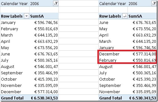
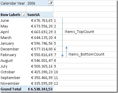
OrderedValues

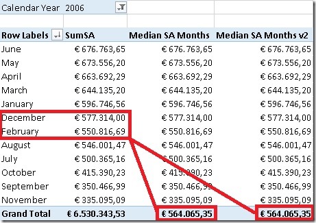
In this example, our set contains 12 items (=months) so we have to find the 2 items in the middle of the ordered set – December and February – and calculate the mean.

So, how can we address this problem using DAX? Most of the posts I mentioned above use some kind of combination of ranking – RANKX() – and filtering – FILTER(). For my approach I will use none of these but use TOPN instead (yes, I really like that function as you probably know if you followed my blog for some time).

In this special case, TOPN() can do both, ranking and filtering for us. But first of all we need to know how many items exist in our set:

Cnt_Months:=DISTINCTCOUNT(‘Date’[Month])


This value will be subsequently used in our next calculations.

To find the value(s) in the middle I use TOPN() twice, first to get the first half of the items (similar to TopCount) and then a second time to get the last values that we need for our median calculation (similar to BottomCount):

TopBottom

As the median calculation is different for even and odd sets, this also has to be considered in our calculation. For both calculations MOD()-function is used to distinguish both cases:

Items_TopCount:=IF(MOD([Cnt_Months],2) = 0,
([Cnt_Months] / 2) + 1,
([Cnt_Months] + 1) / 2)

For an even number of items (e.g. 12) we simply divide the count of items by 2 and add 1 which gives us a (12 / 2) + 1 = 7 for our sample.
For an odd number of items (e.g. 5) we first add 1 to our count of items and then divide by 2 which gives us (5 + 1) / 2 = 3

Items_BottomCount:=IF(MOD([Cnt_Months],2) = 0, 2, 1)

For an even number of items we have to consider the last 2 values whereas for an odd number of items we only have to consider the last value.


These calculations are then used in our median calculation:

Median SA Months:=CALCULATE([SumSA],
TOPN(
[Items_BottomCount],
TOPN(
[Items_TopCount],
VALUES(‘Date’[Month]),
[SumSA]),
[SumSA] * -1))
/
[Items_BottomCount]

As DAX has no built-in BOTTOMN()-function, we need to “abuse” the TOPN() function and multiply the OrderBy-value by “–1” to get the BOTTOMN() functionality. As you can see most of the logic is already handled by our [Items_TopCount] and [Items_BottomCount] measures and this pattern can be reused very easily.


Of course all these calculations can also be combined and the use of IF() can be avoided:

Median SA Months v2:=CALCULATE([SumSA],
TOPN(
2 – MOD([Cnt_Months], 2),
TOPN(
([Cnt_Months] + 1) / 2,
VALUES(‘Date’[Month]),
[SumSA]),
[SumSA] * -1))
/
(2 – MOD([Cnt_Months], 2))

Note: for an even population ([Cnt_Months] + 1) / 2 returns X.5 which is automatically rounded up when it is used in a function that expects a whole number. In our example this is what happens: (12 + 1) / 2 = 6.5 –> 7

These are the final results:

FinalResults


Additional content:

We could also use AVERAGEX() to calculate our median but I think that it is some kind of overhead to use AVERAGEX() just to divide by “1” or “2” depending on the number of items that our TOPN-functions return:

Median SA Months AvgX:=AVERAGEX(
TOPN(
2-MOD([Cnt_Months], 2),
TOPN(
([Cnt_Months] +1) / 2,
VALUES(‘Date’[Month]),
[SumSA]),
[SumSA] * -1),
[SumSA])


As you can see there are various approaches to calculate the median, its up to you which on you like most. I have not tested any of them in terms of performance over bigger sets – this may be topic for an upcoming post.


Download Final Model (Office 2013!)

Another Post about Calculating New and Returning Customers – Part 2

In my previous post I showed a new approach on how to calculate new (and returning) customers in PowerPivot/tabular using DAX. We ended up with a solution where we added the customers first order date as a calculated column to our customer-table. This column was then linked to our date-table with an inactive relationship. The final calculation used USERELATIONSHIP() to make use of this relationship as follows:

New Customers:=CALCULATE(
COUNTROWS(Customer),
USERELATIONSHIP(Customer[FirstOrderDate], ‘Date’[Date]))

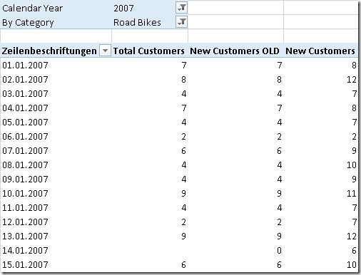
This calculation performs really well as it does not have to touch the fact-table to get the count of new customers. And this is also the issue with the calculation as other filters are not reflected in the calculation:

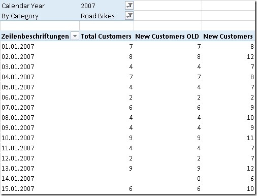
Issue_Old_vs_New

Take row 2 as an example: we have 8 “Total Customers” of which 12 are “New Customers”. Obviously an error in the calculation. The PivotTable is filtered to Category=”Road Bikes” and we have 8 customers on the 2nd of February that bought a road bike. The “New Customers” calculation on the other hand is not related to the Subcategory and shows 12 as in total there were 12 new customers for all products.


To get our calculation working also with other filters we have to somehow relate it to our fact-table. So far we calculated the customers first order date only in the customer table. The customers first order may be related to several fact-rows, e.g. one row for each product the customer bought. Our “New Customers” calculation should only include customers that are active considering also all other filters.

To identify a customers first order in our fact-table we can again use a calculated column and also re-use our previous calculated column in our Customer-table that holds the customers first order date:

=NOT(
ISBLANK(
LOOKUPVALUE(
Customer[CustomerKey],
[CustomerKey],
Customer[FirstOrderDate],
[Order Date]
)))

This returns True for all fact-rows associated with a customers first order and False for all other rows.

The final “New Customers v2” calculation is quite simple then – in addition to the active filters we add a further filter to only select rows that are associated to a customers first order:

New Customers v2:=CALCULATE(
[Total Customers],
‘Internet Sales’[IsCustomersFirstOrder] = TRUE())


And this are the results:

Final_Old_vs_NewV2

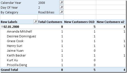
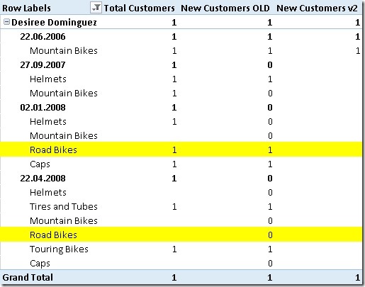
As you can see there are still differences between “New Customers OLD” and “New Customers v2”. But is this really a problem with the new calculation? Lets analyze the issue taking customer “Desiree Dominguez” where we encounter the first difference as an example:

Issue_Analyzed

“Desiree Dominguez” had her first order on the 22th of June in 2006. So she is actually no “new customer” in 2008. The reason why the old calculation counts her as “new customer” is that it was the first time that she bought a product of subcategory “Road Bikes”. Whether this is correct or not is up to your business definition of a “new customer”. According to my experience it is more likely that “Desiree Dominguez” is not counted as a new customer in 2008 and so the “New Customer v2” actually returns the more accurate results.


Additional stuff:

An other option for this calculation is to rank the [Order Date] or [Sales Order Number] for each customer within the fact-table using the calculation below:

=RANKX(
FILTER(
ALL(‘Internet Sales’),
[CustomerKey] = EARLIER([CustomerKey])),
[Order Date],
[Order Date],
1,
DENSE
)

[Order Date] could be replaced by [Sales Order Number]. This makes sense if a customer can have multiple orders per day and you also want to distinguish further by [Sales Order Number]. The new field would also allow new analysis. For example the increase/decrease in sales from the second order compared to the first order and so on.

The “New Customer” calculation in this case would still be similar. We just have to filter on the new calculated column instead:

New Customers v3:=CALCULATE(
[Total Customers],
‘Internet Sales’[CustomersOrderNr] = 1)


Download Final Model (Office 2013!)


The multidimensional model:

The whole logic of extending the fact-table to identify rows that can be associated with a customers first order can also be used in a multidimensional model. Once we prepared the fact-table accordingly the calculations are quite easy. The biggest issues here does not reside in the multidimensional model itself but in the ETL/relational layer as this kind of operation can be quite complex – or better say time-consuming in terms of ETL time.

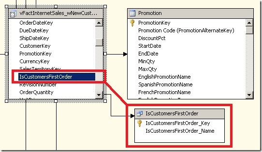
At this point I will not focus on the necessary ETL steps but start with an already prepared fact-table and highlight the extensions that have to be made in the multidimensional model. The fact-table already got extended by a new column called [IsCustomersFirstOrder] similar to the one we created in tabular using a DAX calculated column. It has a value of 1 for rows associated with a customers first order and 0 for all other rows.

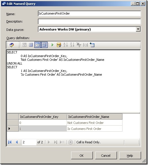
The next thing we have to do is to create a new table in our DSV to base our new dimension on. For simplicity I used this named query:

MD_NamedQuery_Dim

This table is then joined to the new fact-table:

MD_DSV

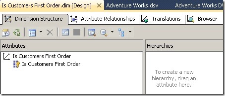
The new dimension is quite simple as it only contains one attribute:

MD_Dimension

You may hide the whole dimension in the end as it may only be used to calculate our “new customers” and nowhere else and may only confuse the end-user.


Once we have added the dimension also to our cube we can create a new calculated measure to calculate our “new customers” as follows:

CREATE MEMBER CURRENTCUBE.[Measures].[New Customers] AS (
[Measures].[Customer Count],
[Is Customers First Order].[Is Customers First Order].&[1]
), ASSOCIATED_MEASURE_GROUP = ‘Internet Customers’
, FORMAT_STRING = ‘#,##0’;

The calculation is based on the existing [Customer Count]-measure which uses DistinctCount-aggregation. Similar to DAX with just extend the calculation by further limiting the cube-space where “Is customers First Order” = 1.

This approach also allows you to create aggregations if necessary to further improve performance. So this is probably also the best way in terms of query-performance to calculate the count of new customers in a multidimensional model.

Another Post about Calculating New and Returning Customers

I know, this topic has already been addressed by quite a lot of people. Chris Webb blogged about it here(PowerPivot/DAX) and here(SSAS/MDX), Javier Guillén here, Alberto Ferrari mentions it in his video here and also PowerPivotPro blogged about it here. Still I think that there are some more things to say about it. In this post I will review the whole problem and come up with a new approach on how to solve this issue for both, tabular and multidimensional models with the best possible performance I could think of (hope I am not exaggerating here  🙂 )

OK, lets face the problem of calculating new customers first and define what a new customer for a given period actually is:

A new customer in Period X is a customer that has sales in Period X but did not have any other sales ever before. If Period X spans several smaller time periods
(e.g. Period X=January contains 31 days) then there must not be any sales before the earliest smaller time period (before 1st of January) for this customer to be counted as a new customer.

According to this definition the common approach can be divided into 2 steps:
1) find all customers that have sales till the last day in the selected period
2) subtract the number of customers that have sales till the day before the first day in the
selected period


First of all we need to create a measure that calculates our distinct customers.
For tabular it may be a simple calculated measure on your fact-table:

Total Customers:=DISTINCTCOUNT(‘Internet Sales’[CustomerKey])

For multidimensional models it should be a physical distinct count measure in your fact-table, ideally in a separate measure group.

How to solve 1) in tabular models

This is also straight forward as DAX has built-in functions that can do aggregation from the beginning of time. We use MAX(‘Date’[Date]) to get the last day in the current filter context:

Customers Till Now:=CALCULATE(
[Total Customers],
DATESBETWEEN(
‘Date’[Date],
BLANK(),
MAX(‘Date’[Date])))


How to solve 2) in tabular models

This is actually the same calculation as above, we only use MIN to get the first day in the current filter context and also subtractt “1” to get the day before the first day.

Previous Customers:=CALCULATE(
[Total Customers],
DATESBETWEEN(
‘Date’[Date],
BLANK(),
MIN(‘Date’[Date])-1))


To calculate our new customers we can simply subtract those two values:

New Customers OLD:=[Customers Till Now]-[Previous Customers]


How to solve 1) + 2) in multidimensional models

Please refer to Chris Webb’s blog here. The solution is pure MDX and is based on a combination of the range-operator “{null:[Date].[Calendar].currentmember}”, NONEMPTY() and COUNT().


Well, so far nothing new.


So lets describe the solution that I came up with. It is based on a different approach. To make the approach easily understandable, we have to rephrase the answer to our original question “What are new customers”?”:

A new customer in Period X is a customer that has his first sales in Period X.

According to this new definition we again have 2 steps:
1) Find the first date with sales for each customer
2) count the customers that had their first sales in the selected period

I will focus on tabular models. For multidimensional models most of the following steps have to be solved during ETL.


How to solve 1) in tabular models

This is pretty easy, we can simply create a calculated column in our Customer-table and get the first date on which the customer had sales:

=CALCULATE(MIN(‘Internet Sales’[Order Date]))


How to solve 2) in tabular models

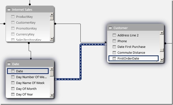
The above create calculated column allows us to relate our ‘Date’-table directly to our ‘Customer’-table. As there is already an existing relationship between those tables via ‘Internet Sales’ we have to create an inactive relationship at this point:

Customer_Date_Relationship

Using this new relationship we can very easy calculate customers that had their first sales in the selected period:

New Customers:=CALCULATE(
COUNTROWS(Customer),
USERELATIONSHIP(Customer[FirstOrderDate], ‘Date’[Date]))


Pretty neat, isn’t it?
We can use COUNTROWS() opposed to a distinct count measure as our ‘Customer’-table only contains unique customers – so we can count each row in the current filter context.
Another nice thing is that we do not have to use any Time-Intelligence function like DATESBETWEEN which are usually resolved using FILTER that would iterate over the whole table. Further it also works with all columns of our ‘Date’-table, no matter whether it is [Calendar Year], [Fiscal Semester] or [Day Name of Week]. (Have you ever wondered how many new customers you acquired on Tuesdays? 🙂 )   And finally, using USERELATIONSHIP allows us to use the full power of xVelocity as native relationships are resolved there.


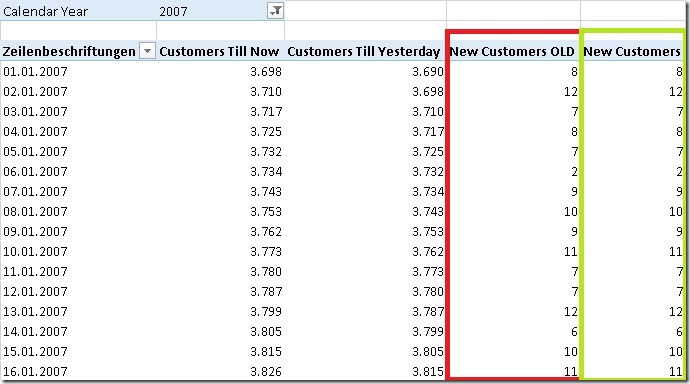
The results are of course the same as for [New Customers OLD]:

Result_Old_vs_New


Though, there are still some issues with this calculation if there are filters on other tables:

Issue_Old_vs_New

As you can see, our new [New Customers] measure does not work in this situation as it is only related to our ‘Date’-table but not to ‘Product’.

I will address this issue in a follow-up post where I will also show how the final solution can be used for multidimensional models – Stay tuned!

Download Final Model (Office 2013!)


UPDATE: Part2 can be found here