Error-handling in Power Query

Data is the daily bread-and-butter for any analyst. In order to provide good results you also need good data. Sometimes this data is very well prepared beforehand and you can use it as it is but it is also very common that you need to prepare and transform the data on your own. To do this Microsoft has introduced Power Query (on tool of the Power BI suite). Power Query can be used to extract, transform and load data into Excel and/or Power Pivot directly.

When using any data you usually know what the data looks like and what to expect from certain columns – e.g. a value is delivered as a number, a text contains exactly 4 characters, etc.
Though, sometimes this does not apply for all rows of that dataset and your transformation logics may cause errors because of that. In order to avoid this and still have a clean data load you need to handle those errors. Power Query offers several options to this which I will elaborate in this post.

This is the sample data I will use for the following samples:

A B C
1 4 AXI23
2 5 TZ560
NA 6 UP945

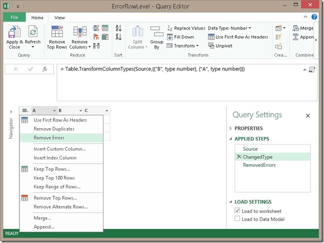
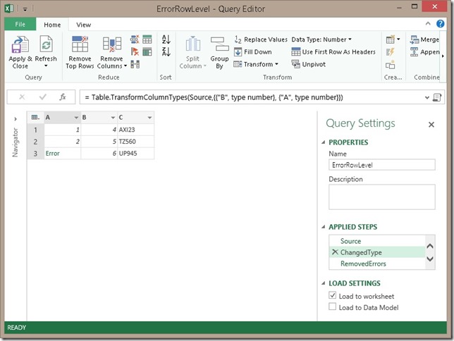
we will perform simple transformations and type casts on this table to generate some errors:

Prepare_ChangeType

Error-handling on row-level

This is the easiest way of handling errors. Whenever a transformation causes an error, we can simply remove the whole row from the result set:

RowLevel_RemoveErrors

This will generate the following result table:

A B C
1 4 AX312
2 5 TZ560

As you can see, the third row was simply removed. This is the easiest way on how to remove errors from your result set but of course this may not be what you want as those removed rows may contain other important information in other columns! Assume you want to calculate the SUM over all values in column B. As we removed the third row we also removed a value from column B and the SUM is not the same as without the error-handling (9 vs. 15)!

Error-handling on cell-level

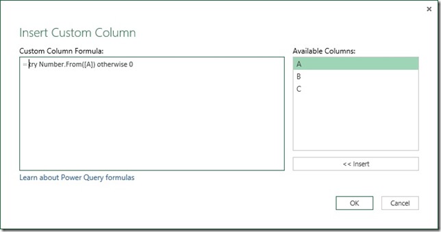
As we now know that column A may result in an error, we can handle this error during our transformation steps. As “NA” could not be converted to a number we see Error as result for that column. Clicking on it gives use some more details on the error itself. To handle this error we need to create a new calculated column where we first check if the value can be converted to a number and otherwise return a default numeric value:

RowLevel_RemoveErrors_CalcColumn

The M-function that we use is “try <expressions to try> otherwise <default if error>” which is very similar to a try-catch block in C#. If the expression causes an error, the default will be used instead. Details on the try-expression can be found in the Microsoft Power Query for Excel Formula Language Specification (PDF) which can be found here and is a must read for everyone interested in the M language.

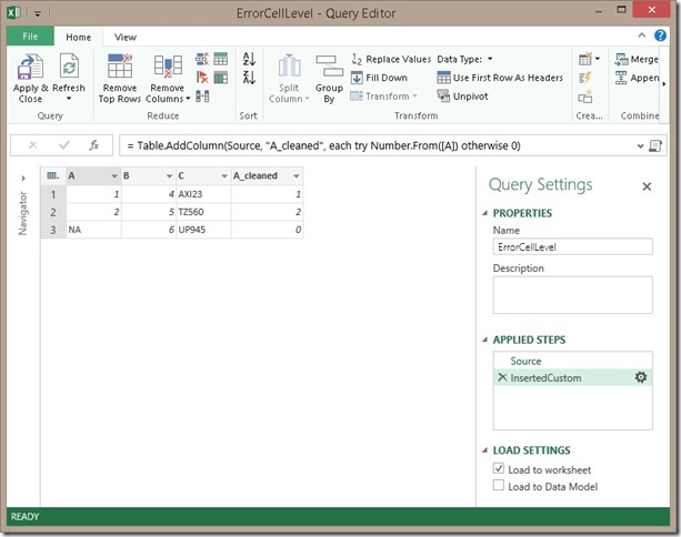
CellLevel_HandleError

We could further replace our column A by the new column A_cleaned to hide this error handling transformation.

A B C A_cleaned
1 4 AXI23 1
2 5 TZ560 2
NA 6 UP945 0

Error-handling on cell-level with error details

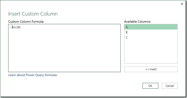
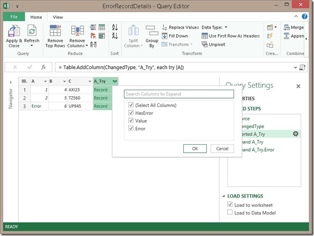
There may also be cases where it is OK to have one of this errors but you need/want to display the cause of the error so that a power user may correct the source data beforehand. Again we can use the try-function, but this time without the otherwise-clause. This will return a record-object for each row:

RowLevel_ShowErrors_CalcColumn

RowLevel_ShowErrors_Result1

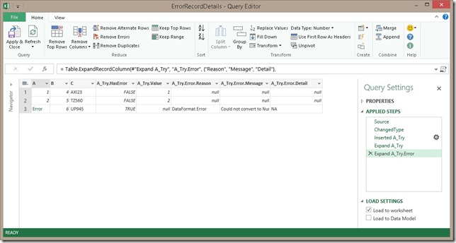
After expanding the A_Try column and also the A_Try.Error column we will get all available information on the error:

RowLevel_ShowErrors_Result2

A B C A_Try.HasError A_Try.Value A_Try.Error.Reason A_Try.Error.Message A_Try.Error.Detail
1 4 AXI23 FALSE 1
2 5 TZ560 FALSE 2
6 UP945 TRUE DataFormat.Error Could not convert to Number. NA

As you can see we get quite a lot of columns here. We could e.g. use A_Try.HasError to filter out error rows (similar to error-handling on row-level) or we could use it in a calculated column to mimic error-handling on cell-level. What you want to do with all the information is up to you, but in case you don’t need it you should remove all unnecessary columns.

Downloads:

Power Query Error Handling Workbook: Power Query Error Handling.xlsx
Using Power Query to analyze SSAS Disk Usage

Some time ago Bob Duffy blogged about on how to use Power Pivot to analyze the disk usage of multidimensional Analysis Services models (here). He uses a an VBA macro to pull meta data like filename, path, extension, etc. from the file system or to be more specific from the data directory of Analysis Services. Analysis Services stores all its data in different files with specific extensions so it is possible to link those files to multidimensional objects in terms of attributes, facts, aggregations, etc. Based on this data we can analyze  how our data is distributed. Do we have too big dimensions? Which attribute uses the most space? Do our facts consume most of the space (very likely)? If yes, how much of it is real data and how big are my aggregations – if they are processed at all?!? – These are very common and also important things to know for an Analysis Services developer.

So Bob Duffy’s solution can be really useful. The only thing I did not like about it was the fact that it uses a VBA macro to get the data. This made me think and I came up with the idea of using Power Query to get this data. Btw, make sure to check out the latest release, there have been a lot of improvements recently!

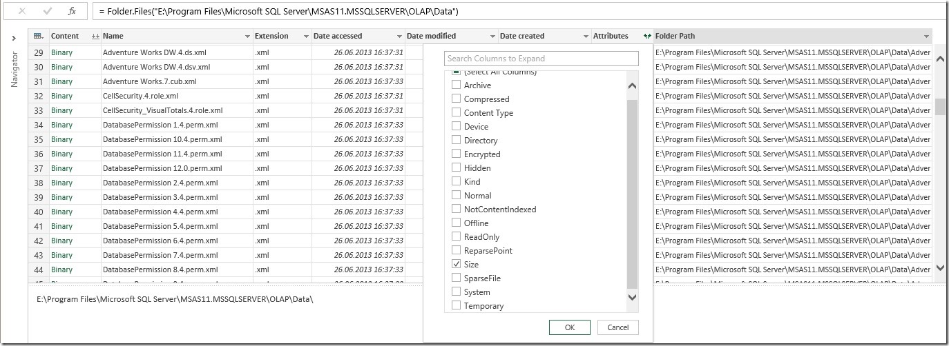
With Power Query you have to option to load multiple files from a folder and also from its sub folders. When we do this on our Analysis Services data directory, we get a list of ALL files together with their full path, filename, extension and most important in this case their size which can be found by expanding the Attributes-record:
PQ_Source_FileList

The final Power Query does also a lot of other things to prepare the data so it can be later joined to our FileExtensions-table that holds detailed information for each file extension. This table currently looks like below but can be extended by any other columns that may be necessary and/or useful for you:

FileType FileType_Description ObjectType ObjectTypeSort ObjectTypeDetails
ahstore Attribute Hash Store Dimensions 20 Attribute
asstore Attribute String Store Dimensions 20 Attribute
astore Attribute Store Dimensions 20 Attribute
bsstore BLOB String Store Dimensions 20 BLOB
bstore BLOB Store Dimensions 20 BLOB
dstore Hierarchy Decoding Store Dimensions 20 Hierarchy
khstore Key Hash Store Dimensions 20 Key
ksstore Key String Store Dimensions 20 Key
kstore Key Store Dimensions 20 Key
lstore Structure Store Dimensions 20 Others
ostore Order Store Dimensions 20 Others
sstore Set Store Dimensions 20 Others
ustore ustore Dimensions 20 Others
xml XML Configuration 999 Configuration
fact.data Basedata Facts 10 Basedata
fact.data.hdr Basedata Header Facts 10 Basedata
fact.map Basedata Index Facts 10 Basedata
fact.map.hdr Basedata Index Header Facts 10 Basedata
rigid.data Rigid Aggregation Data Facts 10 Aggregations
rigid.data.hdr Rigid Aggregation Data Header Facts 10 Aggregations
rigid.map Rigid Aggregation Index Facts 10 Aggregations
rigid.map.hdr Rigid Aggregation Index Header Facts 10 Aggregations
flex.data Flexible Aggregation Data Facts 10 Aggregations
flex.data.hdr Flexible Aggregation Data Header Facts 10 Aggregations
flex.map Flexible Aggregation Index Facts 10 Aggregations
flex.map.hdr Flexible Aggregation Index Header Facts 10 Aggregations
string.data String Data (Distinct Count?) Facts 10 Basedata
cnt.bin Binary Configuration 999 Binaries
mrg.ccmap mrg.ccmap DataMining 999 DataMining
mrg.ccstat mrg.ccstat DataMining 999 DataMining
nb.ccmap nb.ccmap DataMining 999 DataMining
nb.ccstat nb.ccstat DataMining 999 DataMining
dt dt DataMining 999 DataMining
dtavl dtavl DataMining 999 DataMining
dtstr dtstr DataMining 999 DataMining
dmdimhstore dmdimhstore DataMining 999 DataMining
dmdimstore dmdimstore DataMining 999 DataMining
bin Binary Configuration 999 Binaries
OTHERS Others Others 99999 Others

As you can see the extension may contain 1, 2 or 3 parts. The more parts the more specific this file extension is. If you checked the result of the Power Query it also contains 3 columns, FileExtension1, FileExtension2 and FileExtension3. To join the two tables we first need to load both tables into Power Pivot. The next step is to create a proper column on which we can base our relationship. If the 3-part extension is found in the file extensions table, we use it, otherwise we check the 2-part extension and afterwards the 1-part extension and in case nothing matches we use “OTHERS”:

=SWITCH(TRUE(),
CONTAINS(FileTypes, FileTypes[FileType], [FileExtension3]), [FileExtension3],
CONTAINS(FileTypes, FileTypes[FileType], [FileExtension2]), [FileExtension2],
CONTAINS(FileTypes, FileTypes[FileType], [FileExtension1]), [FileExtension1],
"OTHERS")

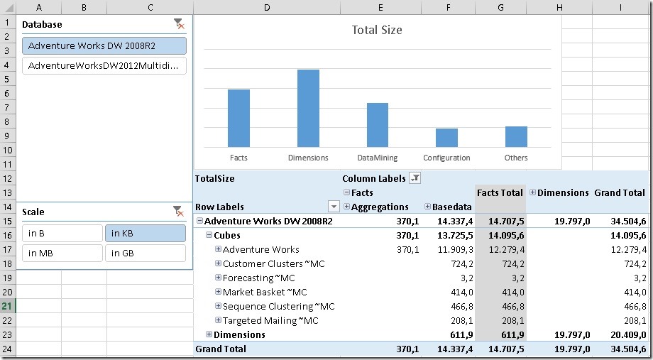
Then we can create a relationship between or PQ table and our file extension table. I also created some other calculated columns, hierarchies and measures for usability. And this is the final outcome:
PivotTable_Report

You can very easily see, how big your facts are, the distribution between base-data and Aggregations, the Dimensions sizes and you can drill down to each individual file! You can of course also create a Power View report if you want to. All visualizations are up to you, this is just a very simple example of a report.

Enjoy playing around with it!

Downloads:
(please note that I added a filter on the Database name as a last step of the Power Query to only show Adventure Works databases! In order to get all databases you need to remove this filter!)

SSAS Disk Analysis Workbook: SSAS_DiskAnalysis.xlsx
SAP HANA’s Big Data Scenario with Power BI

While browsing the web for any BI related topics I recently came across this blog post about SAP HANA and how it can be used to analyze Big Data. Its actually pretty cool, SAP together with Amazon Web Services (AWS) offer a free try out of their tools for 4 hours which you can use to rebuild a predefined demo. The demo itself is very well explained and document with videos and scripts and gives some good insights on how to deal with Big Data in SAP HANA. Basically it is divided into 3 steps:
1) Load Wikipedia data (Pagehits, etc.) from Hadoop/Hive (~2GB of flatfiles)
2) Create a data mart with SAP HANA
3) Analyze results with SAP Lumira

Having done a lot recently with Power BI and its tools I asked myself if this would also be possible with Power BI? So I first did the demo on SAP HANA and afterwards I was quite sure that I could do the same also with Power BI.

And this was the initiation of this blog post where we will do the same demo but instead of SAP HANA we will use only tools of the Power BI suite. Basically we only use 3 of our Power tools:
1) Power Query to load the data
2) Power Pivot to build the “data mart”
3) Power View to analyze the data

First of all we need to load the data. The demo uses data from Wikipedia where for each year, month, day and hour the number of pagehits and bytesdownloaded are monitored per page: http://dumps.wikimedia.org/other/pagecounts-raw/

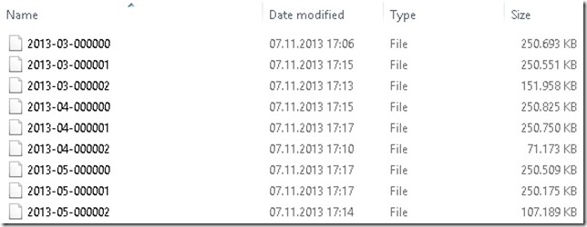
This data was then moved to a Hadoop/Hive cluster on AWS S3 store which was made public available. The transformed files can be downloaded here (~250MB per file):
http://wikipedia-pagecounts-hive-results.s3.amazonaws.com/year=2013/month=03/000000
http://wikipedia-pagecounts-hive-results.s3.amazonaws.com/year=2013/month=03/000001
http://wikipedia-pagecounts-hive-results.s3.amazonaws.com/year=2013/month=03/000002
http://wikipedia-pagecounts-hive-results.s3.amazonaws.com/year=2013/month=04/000000
http://wikipedia-pagecounts-hive-results.s3.amazonaws.com/year=2013/month=04/000001
http://wikipedia-pagecounts-hive-results.s3.amazonaws.com/year=2013/month=04/000002
http://wikipedia-pagecounts-hive-results.s3.amazonaws.com/year=2013/month=05/000000
http://wikipedia-pagecounts-hive-results.s3.amazonaws.com/year=2013/month=05/000001
http://wikipedia-pagecounts-hive-results.s3.amazonaws.com/year=2013/month=05/000002

FileList

Once we have downloaded the files we can start loading them using Power Query’s “Load from Folder” source. It is basically textdata which needs to be split into several columns first. The delimiter used is 0x0001 which in Power Query’s M-language needs to be resolved to “#(0001)”:

= Table.SplitColumn(ImportedText ,"Column1",
    Splitter.SplitTextByDelimiter("#(0001)"),
    {"Column1.1", "Column1.2", "Column1.3", "Column1.4",
     "Column1.5", "Column1.6", "Column1.7", "Column1.8"})

The columns are defined as PROJECTCODE, PAGENAME, YEAR, MONTH, DAY, HOUR, PAGEHITCOUNTFORHOUR and BYTESDOWNLOADEDFORHOUR where PROJECTCODE can be further split into language code and the real project code. There is some more logic which I will not explain in detail like error handling, data conversions, etc., which are similar to what is done in the SAP HANA demo.

This is the final M-script I came up with:

let
    Source = Folder.Files("E:\SAP\Big Data"),
    FilteredRows = Table.SelectRows(Source, each ([Extension] = "")),
    CombinedBinaries = Binary.Combine(FilteredRows[Content]),
    ImportedText = Table.FromColumns({Lines.FromBinary(CombinedBinaries)}),
    SplitColumnDelimiter = Table.SplitColumn(ImportedText ,"Column1",Splitter.SplitTextByDelimiter("#(0001)"),{"Column1.1", "Column1.2", "Column1.3", "Column1.4", "Column1.5", "Column1.6", "Column1.7", "Column1.8"}),
    ChangedType = Table.TransformColumnTypes(SplitColumnDelimiter,{{"Column1.1", type text}, {"Column1.2", type text}, {"Column1.3", type number}, {"Column1.4", type number}, {"Column1.5", type number}, {"Column1.6", type number}, {"Column1.7", type number}, {"Column1.8", type number}}),
    SplitColumnDelimiter1 = Table.SplitColumn(ChangedType,"Column1.1",Splitter.SplitTextByDelimiter("."),{"Column1.1.1", "Column1.1.2"}),
    ChangedType1 = Table.TransformColumnTypes(SplitColumnDelimiter1,{{"Column1.1.1", type text}, {"Column1.1.2", type text}}),
    ReplacedValue = Table.ReplaceValue(ChangedType1,null,"wp",Replacer.ReplaceValue,{"Column1.1.2"}),
    InsertedCustom = Table.AddColumn(ReplacedValue, "PageHitsPerHour", each try Number.From([Column1.7]) otherwise 0),
    InsertedCustom1 = Table.AddColumn(InsertedCustom, "BytesDownloadedPerHour", each try Number.From([Column1.8]) otherwise 0),
    RemovedColumns = Table.RemoveColumns(InsertedCustom1,{"Column1.7", "Column1.8"}),
    RenamedColumns = Table.RenameColumns(RemovedColumns,{{"Column1.3", "Year"}, {"Column1.4", "Month"}, {"Column1.5", "Day"}, {"Column1.6", "Hour"}, {"Column1.2", "PageName"}, {"Column1.1.1", "LanguageCode"}, {"Column1.1.2", "ProjectCode"}}),
    InsertedCustom2 = Table.AddColumn(RenamedColumns, "Date", each #date([Year],[Month],[Day])),
    ChangedType2 = Table.TransformColumnTypes(InsertedCustom2,{{"PageHitsPerHour", type number}, {"BytesDownloadedPerHour", type number}, {"Date", type date}}),
    FilteredRows1 = Table.SelectRows(ChangedType2, each [PageHitsPerHour] < 53000000)
in
    FilteredRows1

If you also did the demo on SAP HANA you found some quality issues in the data why you needed to remove rows with more than 53,000,000 PageHitsPerHour as this 5 rows mess up the whole analysis. The above M-script already handles this (last statement).

There are some more important things to mention here. First of all we are dealing with about 37M rows, so loading to datasheet will not work. Instead we need to load the data directly into Power Pivot. I had several memory issues when using 32bit Excel but after switching to a 64bit Excel everything went just fine. The import itself takes about 15 minutes which I think is OK for roughly 2GB of data and 37M rows. 

Once the data is loaded into Power Pivot we need to load some additional data which are basically our lookup/dimension tables. They can also be imported from Wikipedia, in this case directly from the web:
http://wikipedia-proj-lang-codes.s3.amazonaws.com/UniqueProjectCodes.csv
http://wikipedia-proj-lang-codes.s3.amazonaws.com/UniqueLanguageCodes.csv

Both are very simple tables with only two columns. Again we can use Power Query to import them and add them to our Power Pivot data model.

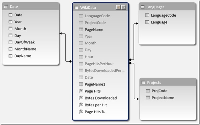
The last thing to add is a time-dimension.SAP HANA has its predefined time-dimension. In the case of Power BI I simply used a linked table in Excel that holds all necessary days or actually all days of 2013. Adding all those tables and linking them we end up with this pretty simple Power Pivot model:

PowerPivot_Diagram

This is very similar to what you create during the demo as an analytical view in SAP HANA so both approaches are very similar here.

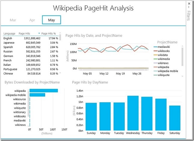
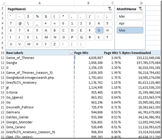
Now that the model is set up we can do our analysis using Power View and classic Excel Pivot Tables:

PowerView_Analysis

PivotTable_Report

All together it took me about 2 hours to build the whole solution of which it took about 1h to download and process the data. The final workbook containing all the data has ~500MB which is mainly because of the PageName column which contains a high number of unique values which cannot be compressed very well. After removing the PageName column and some further tuning of the datamodel for compression I could bring the size down to 148 MB. This is quite OK – in numbers this is a compression of 12 from originally 1.74 GB

I hope you understand that I could not attach the whole workbook, instead I created a smaller workbook with only 50k rows by adding a TOP filter in the Power Query. This workbook can be downloaded below.

As I showed in this post, Power BI is capable of handling this kind of data very well. Both, in terms of data volume and also in terms of the type of data (unstructured/semi-structured data). Once the data is loaded into Power Pivot it can be analyzed just like any other data source using all Excel reporting capabilities.

Downloads:
Sample Excel Sheet: Wikidata_small.xlsx
Demo Script SAP HANA: Demo Script SAP HANA.docx
Power Query M-Script: Power Query M-Script.docx

DAX vs. MDX: DataMembers in Parent-Child Hierarchies

Recently when browsing the MSDN PowerPivot Forums I came across this thread where the question was ask on how to show the value which is directly linked to an element in a parent-child hierarchy instead of the aggregation of all "children". In this post I am going to address this problem finally showing a proper solution.


First of all I would like to start with some background to so called "datamembers". The term "datamember" originates from parent-child hierarchies in multidimensional models. It is a dummy-member that is created automatically below each hierarchy-node to hold values that are linked to a node-member directly. This is of course only possible for parent-child hierarchies.

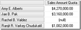
Take the following MDX-Query for example:

SELECT
[Measures].[Sales Amount Quota] ON 0,
Descendants(
    [Employee].[Employees].&[290],
    1,
    SELF_AND_BEFORE) ON 1
FROM [Adventure Works]
WHERE [Date].[Calendar].[Calendar Year].&[2006]

HiddenDatamember

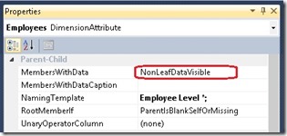
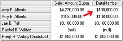
As we can see, the value of "Amy E. Alberts" is not the Sum of its children but has a difference of $108,000.00 This difference is because of the "datamember" that is also a child of every parent-child node which may be hidden. For multidimensional models his behavior can be changed by setting the MembersWithData-Property to "NonLeafDataVisible":

VSProperties


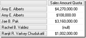
Executing the same query again we now get this results:

VisibleDatamember

Now we see "Amy E. Alberts" twice – the node and the datamember.


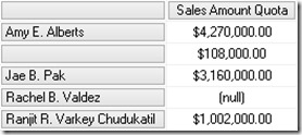
Doing a similar query on a tabular model we will get this result by default:

q4evw0ne

As you can see, we still have the datamember but without any caption. Though, this can of course be changed when you flatten out the hierarchy using DAX by simply replacing BLANK() by "<my datamember caption>" in your calculated columns.


Anyway, this is not the topic of this post but just some background information. Now we will focus on how to query data that is directly associated to a node or its corresponding datamember in MDX and DAX.


MDX:

For MDX this is quite easy as the datamember can be referenced by simply using ".datamember" of a given hierarchy node:

WITH

MEMBER [Measures].[DataMember] AS (
[Measures].[Sales Amount Quota],
[Employee].[Employees].currentmember.datamember
), FORMAT_STRING = 'Currency'

SELECT
{
[Measures].[Sales Amount Quota],
[Measures].[DataMember]
} ON 0,
Descendants(
    [Employee].[Employees].&[290],
    1,
    SELF_AND_BEFORE) ON 1
FROM [Adventure Works]
WHERE [Date].[Calendar].[Calendar Year].&[2006]

DatamemberValue_MDX

The DataMember-Measure only shows values that are directly linked to the current node of the parent-child hierarchy. This is pretty straight forward and very easy to accomplish.


DAX:

In this DAX this problem is a bit more tricky as we do not have that built-in ".datamember" function. Also navigation within hierarchies and parent-child hierarchies itself are not really supported in DAX. Though, there are several blogs out there that describe how to handle parent-child hierarchies by Alberto Ferrari (here) and Kasper de Jonge (here). Based on these solutions we can create our datamember-calculation.

First (and only) thing we need is to add a calculated column that stores the path depth of the current row. This can be achieved by using this formula:

=PATHLENGTH(
    PATH(
        Employee[EmployeeKey],
        Employee[ParentEmployeeKey]
    )
)


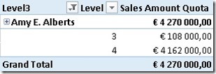
Using our previous example and selecting "Amy E. Alberts" together with our new column we get this:

CalculatedColumn_Level

As we can see there are two different Levels below "Amy E. Alberts" where Level=3 holds our datamember-value and Level=4 holds all the other values (=real child members). Lets add a calculated measure to help you make the final calculation more understandable:

MinLevel:=MIN(Employee[Level])

Calculation_MinLevel

So, for our [DataMember]-calculation we simply have to extend the context to only include rows where [Level] = [MinLevel]

DataMember:=CALCULATE(
SUM('Sales Quota'[Sales Amount Quota]),
FILTER('Employee',
    'Employee'[Level] = [MinLevel]))

CalculationNotWorking_DAX

Well, obviously our calculation is not returning the expected results. This is because of a very common pitfall which I am also very prone to. Whenever a calculated measure is used within an other calculated measure, a CALCULATE() gets wrapped around it thereby taking over the current context. In our case this means that ‘Employee'[Level] will always be the same as [MinLevel] as [MinLevel] gets evaluated for each row and doing MIN() on only one row of course always returns the value of the current row which we compared it to!

To solve this issue we have to place the original [MinLevel]-calculation directly into our [DataMember]-calculation:

DataMember:=CALCULATE(
SUM('Sales Quota'[Sales Amount Quota]),
FILTER('Employee',
    'Employee'[Level] = MIN(Employee[Level])))

CalculationWorking_DAX

This change finally makes the calculation return the correct results also when browsing using the hierarchy:

DatamemberValue_DAX


Even though DAX is not very good in handling hierarchies, the [DataMember]-calculation can be accomplished quite easily. This calculation also works for hierarchies of any depth without needing to adopt it. In terms of performance it may be further improved to the following formula – though the impact will be minor:

DataMember_v2:=CALCULATE(
SUM('Sales Quota'[Sales Amount Quota]),
FILTER(VALUES('Employee'[Level]),
    'Employee'[Level] = MIN(Employee[Level])))


Download Final Model (Office 2013!)

Universal Quantiles Calculation for PowerPivot using DAX

In my last post I showed a new approach on how to calculate the median in PowerPivot using DAX. In the comments the question was raised whether it is possible to make that calculation universal for all kind of Quantiles like Median, Quartiles, Percentiles, etc. and that’s what this post is about.

Lets analyze the final Median calculation from the last post:

Median SA Months:=CALCULATE([SumSA],
TOPN(
2-MOD([Cnt_Months], 2),
TOPN(
([Cnt_Months] + 1) / 2,
VALUES(‘Date’[Month]),
[SumSA]),
[SumSA],
1))
/
(2-MOD([Cnt_Months], 2))


The Median defines the value in the middle of an ordered set. To get the first half (+1 to handle even and odd sets) of the whole we are using TOPN function:

TOPN(
([Cnt_Months] + 1) / 2,
VALUES(‘Date’[Month]),
[SumSA]),

The important part here is the “divide by 2” to split the set in the middle to start our Median calculation. Instead of dividing by 2 we could also multiply by 0.5 where 0.5 would be the separator for our quantile (in this case the Median). This expression can be made dynamic. For the first Quartile we would use 0.25 for the second Quartile (=Median) we would use 0.5 and for the third Quartile we would use 0.75.

I created a little linked table to demonstrate the dynamic approach:

Quantile SortOrder Percentage
Median 1 0.5000
Quartile 1 401 0.2500
Quartile 2 402 0.5000
Quartile 3 403 0.7500
Sextile 1 601 0.1667
Sextile 2 602 0.3333
Sextile 3 603 0.5000
Sextile 4 604 0.6667
Sextile 5 605 0.8333

We also need to add a calculated measure that returns the percentage-value of the currently selected Quantile:

SelectedQuantile:=IF(
HASONEVALUE(Quantiles[Percentage]),
VALUES(Quantiles[Percentage]))


Now we can change our old Median-calculation to be dynamic by using the measure defined above:

Quantile SA Months:=CALCULATE([SumSA],
TOPN(
2 – MOD([Cnt_Months], 2),
TOPN(
ROUNDUP(([Cnt_Months] + 1) * [SelectedQuantile], 0),
VALUES(‘Date’[Month]),
[SumSA]),
[SumSA],
1))
/
(2 – MOD([Cnt_Months], 2))

We also need to explicitly add ROUNDUP() as “([Cnt_Months] + 1) * [SelectedQuantile]” may return any decimal places whereas the previous divide by 2 could only result in a x.5 which was rounded up automatically. And well, that’s all we need to change in order to make the calculation universal for all different Quantiles! The rest is the same logic that I already described for Median calculation.


Download Final Model (Office 2013!)

Calculating Median in PowerPivot using DAX

I just came across this blog post by Bill Anton where he discusses several approaches to calculated the Median of a given set in T-SQL, MDX and DAX. In the end of his post when it comes to the DAX calculation, he references several post by Marco, Alberto and Javier (post1, post2) that already address that kind of calculation in DAX. But he also claims that non of the solutions is “elegant”. Well, reason enough for me to try it on my own and here is what I came up with. Its up to you to decide whether this solution is more elegant than the others or not 🙂

In general, the median calculation always varies depending on the number of items and whether this number is even or odd.
For an even population the median is the mean of the values in the middle:
the median of {3, 5, 7, 9} is is (5 + 7)/2 = 6
For an odd population, the median is the value in the middle:
the median of {3, 5, 9} is 5

In both cases the values have to be ordered before the calculation. Note that it does not make a difference whether the values are sorted in ascending or descending order.

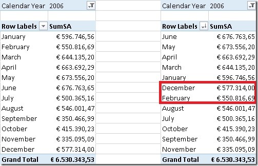
OrderedValues

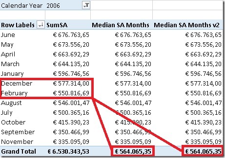
In this example, our set contains 12 items (=months) so we have to find the 2 items in the middle of the ordered set – December and February – and calculate the mean.

So, how can we address this problem using DAX? Most of the posts I mentioned above use some kind of combination of ranking – RANKX() – and filtering – FILTER(). For my approach I will use none of these but use TOPN instead (yes, I really like that function as you probably know if you followed my blog for some time).

In this special case, TOPN() can do both, ranking and filtering for us. But first of all we need to know how many items exist in our set:

Cnt_Months:=DISTINCTCOUNT(‘Date’[Month])


This value will be subsequently used in our next calculations.

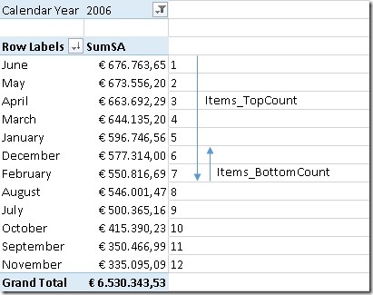
To find the value(s) in the middle I use TOPN() twice, first to get the first half of the items (similar to TopCount) and then a second time to get the last values that we need for our median calculation (similar to BottomCount):

TopBottom

As the median calculation is different for even and odd sets, this also has to be considered in our calculation. For both calculations MOD()-function is used to distinguish both cases:

Items_TopCount:=IF(MOD([Cnt_Months],2) = 0,
([Cnt_Months] / 2) + 1,
([Cnt_Months] + 1) / 2)

For an even number of items (e.g. 12) we simply divide the count of items by 2 and add 1 which gives us a (12 / 2) + 1 = 7 for our sample.
For an odd number of items (e.g. 5) we first add 1 to our count of items and then divide by 2 which gives us (5 + 1) / 2 = 3

Items_BottomCount:=IF(MOD([Cnt_Months],2) = 0, 2, 1)

For an even number of items we have to consider the last 2 values whereas for an odd number of items we only have to consider the last value.


These calculations are then used in our median calculation:

Median SA Months:=CALCULATE([SumSA],
TOPN(
[Items_BottomCount],
TOPN(
[Items_TopCount],
VALUES(‘Date’[Month]),
[SumSA]),
[SumSA] * -1))
/
[Items_BottomCount]

As DAX has no built-in BOTTOMN()-function, we need to “abuse” the TOPN() function and multiply the OrderBy-value by “–1” to get the BOTTOMN() functionality. As you can see most of the logic is already handled by our [Items_TopCount] and [Items_BottomCount] measures and this pattern can be reused very easily.


Of course all these calculations can also be combined and the use of IF() can be avoided:

Median SA Months v2:=CALCULATE([SumSA],
TOPN(
2 – MOD([Cnt_Months], 2),
TOPN(
([Cnt_Months] + 1) / 2,
VALUES(‘Date’[Month]),
[SumSA]),
[SumSA] * -1))
/
(2 – MOD([Cnt_Months], 2))

Note: for an even population ([Cnt_Months] + 1) / 2 returns X.5 which is automatically rounded up when it is used in a function that expects a whole number. In our example this is what happens: (12 + 1) / 2 = 6.5 –> 7

These are the final results:

FinalResults


Additional content:

We could also use AVERAGEX() to calculate our median but I think that it is some kind of overhead to use AVERAGEX() just to divide by “1” or “2” depending on the number of items that our TOPN-functions return:

Median SA Months AvgX:=AVERAGEX(
TOPN(
2-MOD([Cnt_Months], 2),
TOPN(
([Cnt_Months] +1) / 2,
VALUES(‘Date’[Month]),
[SumSA]),
[SumSA] * -1),
[SumSA])


As you can see there are various approaches to calculate the median, its up to you which on you like most. I have not tested any of them in terms of performance over bigger sets – this may be topic for an upcoming post.


Download Final Model (Office 2013!)

Another Post about Calculating New and Returning Customers

I know, this topic has already been addressed by quite a lot of people. Chris Webb blogged about it here(PowerPivot/DAX) and here(SSAS/MDX), Javier Guillén here, Alberto Ferrari mentions it in his video here and also PowerPivotPro blogged about it here. Still I think that there are some more things to say about it. In this post I will review the whole problem and come up with a new approach on how to solve this issue for both, tabular and multidimensional models with the best possible performance I could think of (hope I am not exaggerating here  🙂 )

OK, lets face the problem of calculating new customers first and define what a new customer for a given period actually is:

A new customer in Period X is a customer that has sales in Period X but did not have any other sales ever before. If Period X spans several smaller time periods
(e.g. Period X=January contains 31 days) then there must not be any sales before the earliest smaller time period (before 1st of January) for this customer to be counted as a new customer.

According to this definition the common approach can be divided into 2 steps:
1) find all customers that have sales till the last day in the selected period
2) subtract the number of customers that have sales till the day before the first day in the
selected period


First of all we need to create a measure that calculates our distinct customers.
For tabular it may be a simple calculated measure on your fact-table:

Total Customers:=DISTINCTCOUNT(‘Internet Sales’[CustomerKey])

For multidimensional models it should be a physical distinct count measure in your fact-table, ideally in a separate measure group.

How to solve 1) in tabular models

This is also straight forward as DAX has built-in functions that can do aggregation from the beginning of time. We use MAX(‘Date’[Date]) to get the last day in the current filter context:

Customers Till Now:=CALCULATE(
[Total Customers],
DATESBETWEEN(
‘Date’[Date],
BLANK(),
MAX(‘Date’[Date])))


How to solve 2) in tabular models

This is actually the same calculation as above, we only use MIN to get the first day in the current filter context and also subtractt “1” to get the day before the first day.

Previous Customers:=CALCULATE(
[Total Customers],
DATESBETWEEN(
‘Date’[Date],
BLANK(),
MIN(‘Date’[Date])-1))


To calculate our new customers we can simply subtract those two values:

New Customers OLD:=[Customers Till Now]-[Previous Customers]


How to solve 1) + 2) in multidimensional models

Please refer to Chris Webb’s blog here. The solution is pure MDX and is based on a combination of the range-operator “{null:[Date].[Calendar].currentmember}”, NONEMPTY() and COUNT().


Well, so far nothing new.


So lets describe the solution that I came up with. It is based on a different approach. To make the approach easily understandable, we have to rephrase the answer to our original question “What are new customers”?”:

A new customer in Period X is a customer that has his first sales in Period X.

According to this new definition we again have 2 steps:
1) Find the first date with sales for each customer
2) count the customers that had their first sales in the selected period

I will focus on tabular models. For multidimensional models most of the following steps have to be solved during ETL.


How to solve 1) in tabular models

This is pretty easy, we can simply create a calculated column in our Customer-table and get the first date on which the customer had sales:

=CALCULATE(MIN(‘Internet Sales’[Order Date]))


How to solve 2) in tabular models

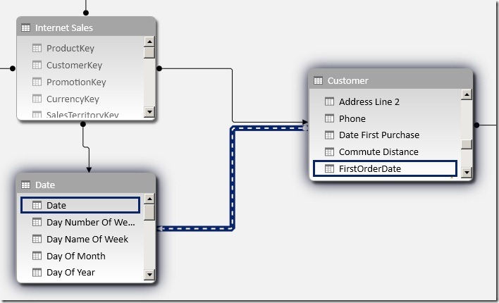
The above create calculated column allows us to relate our ‘Date’-table directly to our ‘Customer’-table. As there is already an existing relationship between those tables via ‘Internet Sales’ we have to create an inactive relationship at this point:

Customer_Date_Relationship

Using this new relationship we can very easy calculate customers that had their first sales in the selected period:

New Customers:=CALCULATE(
COUNTROWS(Customer),
USERELATIONSHIP(Customer[FirstOrderDate], ‘Date’[Date]))


Pretty neat, isn’t it?
We can use COUNTROWS() opposed to a distinct count measure as our ‘Customer’-table only contains unique customers – so we can count each row in the current filter context.
Another nice thing is that we do not have to use any Time-Intelligence function like DATESBETWEEN which are usually resolved using FILTER that would iterate over the whole table. Further it also works with all columns of our ‘Date’-table, no matter whether it is [Calendar Year], [Fiscal Semester] or [Day Name of Week]. (Have you ever wondered how many new customers you acquired on Tuesdays? 🙂 )   And finally, using USERELATIONSHIP allows us to use the full power of xVelocity as native relationships are resolved there.


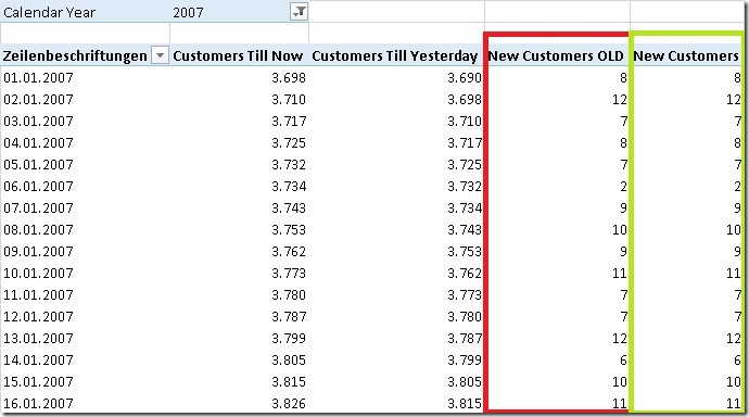
The results are of course the same as for [New Customers OLD]:

Result_Old_vs_New


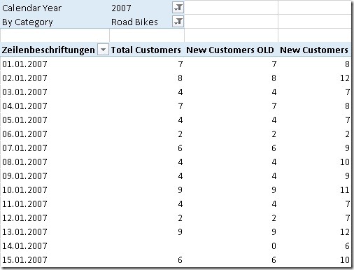
Though, there are still some issues with this calculation if there are filters on other tables:

Issue_Old_vs_New

As you can see, our new [New Customers] measure does not work in this situation as it is only related to our ‘Date’-table but not to ‘Product’.

I will address this issue in a follow-up post where I will also show how the final solution can be used for multidimensional models – Stay tuned!

Download Final Model (Office 2013!)


UPDATE: Part2 can be found here

Fiscal Periods, Tabular Models and Time-Intelligence

I recently had to build a tabular model for a financial application and I would like to share my findings on this topic in this post. Financial applications tend to have “Periods” instead of dates, months, etc. Though, those Periods are usually tied to months – e.g. January = “Period01”, February = “Period02” and so on. In addition to those “monthly periods” there are usually also further periods like “Period13”, “Period14” etc. to store manually booked values that are necessary for closing a fiscal year. To get the years closing value (for a P&L account) you have to add up all periods (Period01 to Period14). In DAX this is usually done by using TOTALYTD() or any similar Time-Intelligence Function.


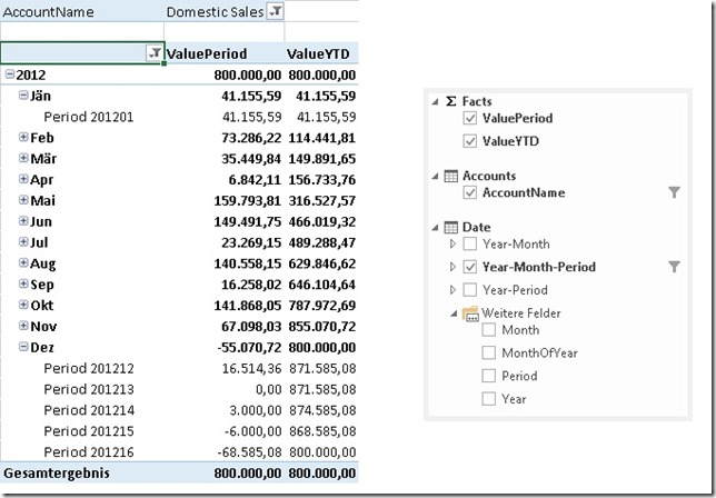
Here is what we want to achieve in the end. The final model should allow the End-user to create a report like this:

DesiredResult

This model allows us to analyze data by Year, by Month and of course also by Period. As you can see also the YTD is calculated correctly using DAX’s built-in Time-Intelligence functions.

However, to make use of Time-Intelligence functions a Date-table is required (more information: Time Intelligence Functions in DAX) but this will be covered later. Lets start off with a basic model without a Date-table.

For testing purposes I created this simple PowerPivot model:

BaseModel 

Sample of table ‘Facts’:

AccountID PeriodID Value
4 201201

41,155.59

2 201201

374,930.01

3 201211

525,545.15

5 201211

140,440.40

1 201212

16,514.36

5 201212

639,998.94

3 201213

-100,000.00

4 201213

20,000.00

5 201214

500,000.00


The first thing we need to do is to add a Date-table. This table should follow these rules:
– granularity=day –> one row for each date
– no gaps between the dates –> a contiguous range of dates
– do not use use the fact-table as your date-table –> always use an independent date-table
– the table must contain a column with the data type “Date” with unique values
– “Mark as Date-table”

A Date-table can be created using several approaches:
– Linked Table
– SQL view/table
– Azure Datamarket (e.g. Boyan Penev’s DateStream)
– …

(Creating an appropriate Date-table is not part of this post – for simplicity i used a Linked Table from my Excel workbook).

I further created calculated columns for Year, Month and MonthOfYear.


At this point we cannot link this table to our facts. We first have to create some kind of mapping between Periods and “real dates”. I decided to create a separate table for this purpose that links one Period to one Date. (Note: You may also put the whole logic into a calculated column of your fact-table.) This logic is straight forward for periods 1 to 11 which are simply mapped to the last (or first) date in that period. For Periods 12 and later this is a bit more tricky as we have to ensure that these periods are in the right order to be make our Time-Intelligence functions work correctly. So Period12 has to be before Period13, Period13 has to be before Period14, etc.

So I mapped Period16 (my sample has 16 Periods) to the 31st of December – the last date in the year as this is also the last period. Period 15 is mapped to the 30th of December – the second to last date. And so on, ending with Period12 mapped to the 27th of December:

PeriodID Date
201101 01/31/2011
201102 02/28/2011
201111 11/30/2011
201112 12/27/2011
201113 12/28/2011
201114 12/29/2011
201115 12/30/2011
201116 12/31/2011
201201 01/31/2012
201202 02/29/2012

I called the table ‘MapPeriodDate’.

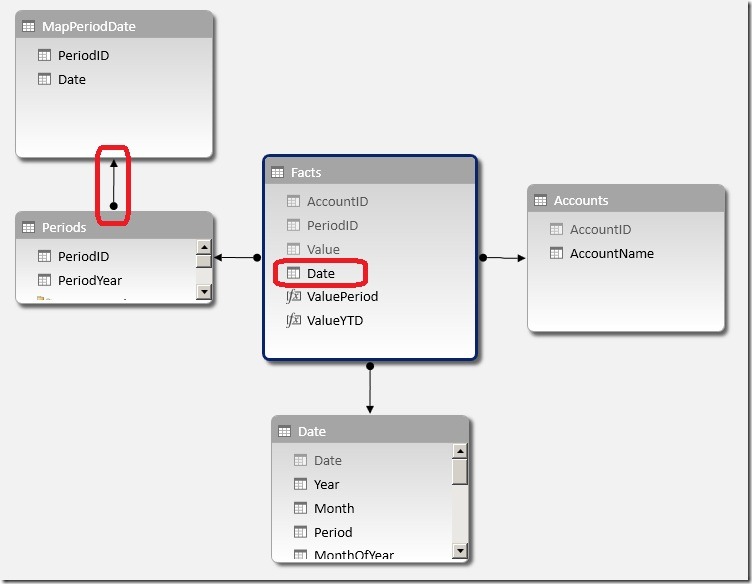
This table is then added to the model and linked to our already existing Period-table (Note: The table could also be linked to the Facts-table directly using PeriodID). This allows us to create a new calculated column in our Facts-table to get the mapping-date for the current Period:

=RELATED(MapPeriodDate[Date])


The new column can now be used to link our Facts-table to our Date-Table:

FinalModel

Please take care in which direction you create the relationship between ‘Periods’ and ‘MapPeriodDate’ as otherwise the RELATED()-function may not work!

Once the Facts-table and the Date-table are connected you may consider hiding the unnecessary tables ‘Periods’ and ‘MapPeriodDate’ as all queries should now use the Date-table. Also the Date-column should be hidden so the lowest level of our Date-table should be [Period].


To get a [Period]-column in our Date-table we have to create some more calculated columns:

[Period_LookUp]
= LOOKUPVALUE(MapPeriodDate[PeriodID], MapPeriodDate[Date], [Date])

this returns the PeriodID if the current date also exists in the MapPeriodDate-table. Note that we only get a value for the last date in a month.


[Period]
= CALCULATE(MIN([Period_LookUp]), DATESBETWEEN('Date'[Date], [Date], BLANK()))

our final [Period]-calculation returns the first populated value of [Period_LookUp] after the current date. The first populated value for dates in January is the 31st which has a value of 201101 – our PeriodID!


The last step is to create our YTD-measures. This is now very easy as we can again use the built-in Time-Intelligence functions with this new Date-table:

ValueYTD:=TOTALYTD(SUM([Value]), 'Date'[Date])

And of course also all other Time-Intelligence functions now work out of the box:

ValuePYTD:=CALCULATE([ValueYTD], DATEADD('Date'[Date], 1, YEAR))


All those calculations work with Years, Months and also Periods and offer the same flexibility that you are used to from the original financial application.


Download Final Model (Office 2013!)

Dynamic ABC Analysis in PowerPivot using DAX

An ABC Analysis is a very common requirement for for business users. It classifies e.g. Items, Products or Customers into groups based on their sales and how much impact they had on the cumulated overall sales. This is done in several steps.

I just published a new version of the Dynamic ABC Analysis at www.daxpatterns.com. The article can be found here.


1) Order products by their sales in descending order
2) Cumulate the sales beginning with the best selling product till the current product
3) Calculate the percentage of the cumulated sales vs. total sales
4) Assign a Class according to the cumulated percentage

Marco Russo already blogged about this here. He does the classification in a calculated column based on the overall sales of each product. As calculated columns are processed when the data is loaded, this is not dynamic in terms of your filters that you may apply in the final report. If, for example, a customer was within Class A regarding total sales but had no sales last year then a report for last year that uses this classification may give you misleading results.

In this blog I will show how to do this kind of calculation on-the-fly always in the context of the current filters. I am using Adventure Works DW 2008 R2 (download) as my sample data and create a dynamic ABC analysis of the products.

The first thing we notice is that our product table is a slowly changing dimension of type 2 and there are several entries for the same product as every change is traced in the same table.

SCD2Table

So we want to do our classification on the ProductAlternateKey (=Business Key) column instead of our ProductKey (=Surrogate Key) column.

First we have to create a ranking of our products:

Rank CurrentProducts:=IF(HASONEVALUE(DimProduct[ProductAlternateKey]),
IF(NOT(ISBLANK([SUM SA])),
RANKX(
CALCULATETABLE(
VALUES(DimProduct[ProductAlternateKey]),
ALL(DimProduct[ProductAlternateKey])),
[SUM SA])))

Check if there is only one product in the current context and that this product also has sales. If this is the case we calculate our rank. We need to do the CALCULATETABLE to do the ranking within the currently applied filters on other columns of the DimProduct-table e.g. if a filter is applied to DimProduct[ProductSubcategoryKey] we want to see our ranking within that selected Subcategory and not against all Products.

I also created a measure [SUM SA] just to simplify the following expressions:

SUM SA:=SUM(FactInternetSales[SalesAmount])


The second step is to create a running total starting with the best-selling product/the product with the lowest rank:

CumSA CurrentProducts:=SUMX(
TOPN(
[Rank CurrentProducts],
CALCULATETABLE(
VALUES(DimProduct[ProductAlternateKey]),
ALL(DimProduct[ProductAlternateKey])),
[SUM SA]),
[SUM SA])

We use a combination of SUMX() and TOPN() here. TOPN() returns the top products ordered by [SUM SA]. Further we use our previously calculated rank to only get the products that have the same or more sales than the current product. For example if the current product has rank 3 we sum up the top 3 products to get our cumulated sum (=sum of the first 3 products) for this product. Again we need to use CALCULATETABLE() to retain other filters on the DimProduct-table.


The third step is pretty easy – we need to calculate percentage of the cumulated sales vs. the total sales:

CumSA% CurrentProducts:=
[CumSA CurrentProducts]
/
CALCULATE([SUM SA], ALL(DimProduct[ProductAlternateKey]))

This calculation is straight forward and should not need any further explanation.

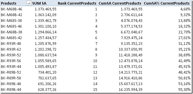
The result of those calculations can be seen here:

Theory


To do our final classification we have to extend our model with a new table that holds our classes and their border-values:

Class LowerBoundary UpperBoundary
A 0 0.7
B 0.7 0.9
C 0.9 1

Class A should contain products which’s cumulated sales are between 0 and 0.7 – between 0% and 70%.
Class B should contain products which’s cumulated sales are between 0.7 and 0.9 – between 70% and 90%.
etc.

(This table can later be extended to support any number of classes and any boundaries between 0% and 100%.)

To get the boundaries of the selected class we create two measures that are later used in our final calculation:

MinLowerBoundary:=MIN([LowerBoundary])
MaxUpperBoundary:=MAX([UpperBoundary])


Our final calculation looks like this:

SA Classified Current:=IF(NOT(ISCROSSFILTERED(Classification[Class])),
[SUM SA],
CALCULATE(
[SUM SA],
FILTER(
VALUES(DimProduct[ProductAlternateKey]),
[MinLowerBoundary] < [CumSA% CurrentProducts]
&& [CumSA% CurrentProducts] <= [MaxUpperBoundary])))

If our Classification-table is not filtered, we just show our [SUM SA]-measure. Otherwise we extend the filter on our DimProduct[ProductAlternateKey] using our classification filtering out all products that do not fall within the borders of the currently selected class.

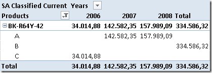
This measure allows us to see the changes of the classification of a specific product e.g. over time:

FinalResults_1

In 2006 our selected product was in Class C. For 2007 and 2008 it improved and is now in Class A. Still, overall it resides in Class B.

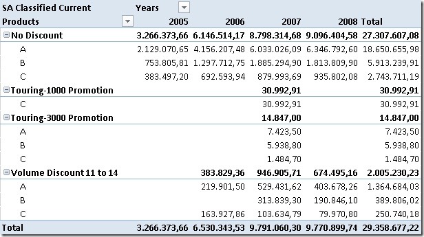
We may also analyze the impact of our promotions on the sales of our classified products:

FinalResults_2

Our Promotion “Touring-1000 Promotion” only had impact on products in Class C so we may consider to stop that promotion and invest more into the other promotions that affect all classes.


The classification can be used everywhere you need it – in the filter, on rows or on columns, even slicers work. The only drawback is that the on-the-fly calculation can take quite some time. If I find some time in the future i may try to further tune them and update this blog-post.


The example workbook can be downloaded here:

Though it is already in Office 2013 format an may not be opened with any previous versions of Excel/PowerPivot.
It also includes a second set of calculations that use the same logic as described above but does all the calculations without retaining any filters on the DimProducts-table. This allows you to filter on Class “A” and ProductSubcategory “Bike Racks” realizing that “Bike Racks” are not a Class “A” product or to see which Subcategories or Categories actually contain Class A, B or C products!

Relationships on columns with non-unique values and how to tune them

If you follow my blog frequently, you may have realized that in many of them I cover scenarios where I need to create relationships on columns with non-unique values. For example when handling SCD2 facts and dimensions or dealing with parallel hierarchies. In all the examples I use a combination of FILTER– and CONTAINS-function to create those non-unique relationships between tables. Recently I ran into performance issues using this approach and was thinking about on how to tune those kind of "relationships".

First of all I was taking a look at the DAX Query Plan using SQL Server Profiler to get some more information on what’s going on inside xVelocity and DAX. I used an calculation from my previous post as an example:

Value_Sender:=
CALCULATE([Value_SUM],
FILTER(
     'Facts',
     CONTAINS(
          'Sender',
          'Sender'[SenderID],
          'Facts'[SenderID]))
)

We had to use this calculation as SenderID was not unique in our Sender-table (and of course also not in our Facts-table). When we tried to create a relationship we got the error

Error

"The relationship cannot be created because each column contains duplicate values. Select at least one column that contains only unique values."

This makes absolutely sense as tabular models natively only support 1:n / n:1 relationships and therefore at least one column has to contain only unique vales.

The calculation from above using FILTER and CONTAINS still allowed us to link our tables on those non-unique column values. The drawback of the calculation is that it may not perform very well as it cannot use the full power of xVelocity that heavily relies on predefined relationships between columns and tables. But in our case we create the relationship on-the-fly not using xVelocity’s full potential. Further, by using CONTAINS, which is not a native xVelocity-function, the engine has to callback to DAX formula engine as we can see in the profiler:

VertiPaq SE Query / 0 – VertiPaq Scan (8 times of which 4 are of subclass Internal)

VertiPaq_SE_Query_CONTAINS

[CallbackDataID(….)] is always an indicator that the xVelocity engine could not resolve the query on its own but had to call functions from the DAX formula engine as Jeffrey Wang described here. This in the end results in poor query performance (at least compared to a pure xVelocity query).

DAX Query Plan / 1 – DAX VertiPaq Logical Plan (just for sake of completeness)

QueryPlan_CONTAINS


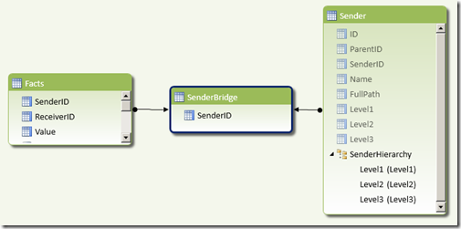
So the key to tune those kind of relationships is to relate the tables at design time to get full xVelocity performance at query time. As the tables cannot be related directly, we have to add an intermediate table containing only unique values – in our case unique SenderIDs. This table can then be used to create 1:n relationships with our Sender and our Facts table

SenderID
TOT
EUROPE
GER
FR
NA
USA
CAN
EXTERNAL
TOT_2
JV
HOLD

If you are using a SQL database as datasource you can simply create a view using SELECT DISTINCT or write the select statement directly in PowerPivot.

Once the table has been added we can create relationships as shown below:

Relationships

This design is similar to a many-to-many design with the only difference that we combined our intermediate table and our bridge table into one single table. The rest is similar to resolving many-to-many relationship as I described here. So once we have created these relationships we can change our calculations as follows:

Value_Sender_Bridge:=
CALCULATE(
     [Value_SUM],
     'SenderBridge',
     'Sender'
)

This calculation can be resolved by the xVelocity engine without any callbacks to DAX formula engine. Taking a look at the profiler trace proves this:

VertiPaq SE Query / 0 – VertiPaq Scan (4 times of which 2 are of subclass Internal)

VertiPaq_SE_Query_CROSSTABLE

None of the Veripaq SE queries used [CallbackDataID(….)] or any other complex function. Only joins have been used which can be handled by the xVelocity engine very easily:

DAX Query Plan / 1 – DAX VertiPaq Logical Plan (just for sake of completeness)

QueryPlan_CROSSTABLE

Also the logical plan could be drastically simplified containing only Sum_Vertipaq and Scan_Vertipaq operators telling us that the query can be executed in pure Vertiscan mode.

Details on Vertipaq operators and Vertiscan mode can be found here.


I have not run a lot of tests on bigger tables yet where I could have compared the overall performance but this may follow in a later post. With this post I just wanted to show how to link tables on columns containing non-unique values.

It would be great if tabular models would support those kind of relationships out of the box and that you can create them like any other relationships using drag&drop in the diagram view. This would have made many of my previous workshops at customers much easier Smile.