When building an enterprise reporting solution with Power BI, a question that always comes up is how to handle translations. Large enterprises operate in various countries where people also speak different languages. So a report should be available in all frequently used languages. Ideally, you just create a report once and then a user can decide (or it is decided for him) in which language the report is displayed.
Power BI only partially supports this scenario and the closest we could get *before field parameters* were introduced is already very well described by Chris Webb’s blog post on Implementing Data (As Well As Metadata) Translations In Power BI – a must-read if you need to deal with translations in Power BI. Another good read on the topic is the blog post Multilingual Reports in Power BI from PBI Guy.
As you will quickly realize, the translation of metadata is already pretty easy as it is baked into the engine. Unfortunately this is not the case when you need to translate actual data values (e.g. product names, …). In the multidimensional version of Analysis Services this just worked like a charm as it was also a native feature but this feature never made it to Analysis Services Tabular Models, Azure Analysis Services or Power BI.
The current approaches when it comes to data and value translations are more workarounds than actual solutions. They probably work fine for small data models and very specific use-cases but usually fall short in performance, usability or maintainability when implemented on a larger scale enterprise models.
The recently introduced Field Parameters in Power BI give us a bit more flexibility here and another potential solution to implement data and value translations in Power BI.
Here is what we want to achieve:
- create a single report only
- support for multiple languages – metadata and column data
- only minor changes to the existing data model
How can Field Parameters help here?
Field Parameters allow you to select the columns you want to display in your report/visual on-the-fly. Based on the selection, the reporting engine decides which physical column(s) it needs to use in the query it generates and sends to the data model.
So we can create a Field Parameter for the different columns that hold the translated data values and already easily switch the language by changing the selection of our Field Parameter. This is how our Filed Parameter would be defined:
Translated ProductName = {
    ("product name", NAMEOF('DimProduct'[EnglishProductName]), 0, "en-US"),
    ("nom du produit", NAMEOF('DimProduct'[FrenchProductName]), 1, "fr-FR"),
    ("nombre de producto", NAMEOF('DimProduct'[SpanishProductName]), 2, "es-SP")
}
I did this for all the fields for which translated values are actually provided. Usually this is just a very small subset of all the available columns!
Translated MonthOfYear = {
    ("MonthName", NAMEOF('DimDate'[EnglishMonthName]), 0, "en-US"),
    ("mois de l'année", NAMEOF('DimDate'[FrenchMonthName]), 1, "fr-FR"),
    ("mes del año", NAMEOF('DimDate'[SpanishMonthName]), 2, "es-SP")
}

Translated DayOfWeek = {
    ("Day Of Week", NAMEOF('DimDate'[EnglishDayNameOfWeek]), 0, "en-US"),
    ("jour de la semaine", NAMEOF('DimDate'[FrenchDayNameOfWeek]), 1, "fr-FR"),
    ("día de la semana", NAMEOF('DimDate'[SpanishDayNameOfWeek]), 2, "es-SP")
}
As you can see, Field Parameters allow you to translate the metadata (first value) and also to define the column to use for the data values (second value, using NAMEOF() function).
To change all field parameters at once I introduced an additional 4th column that holds the culture/language of the current row which is then linked to another static DAX table that is defined as follows:
Language = DATATABLE("Culture", STRING, {{"en-US"}, {"fr-FR"}, {"es-SP"}})
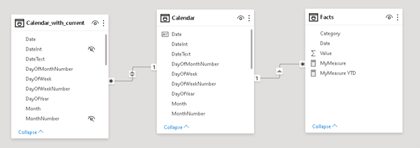
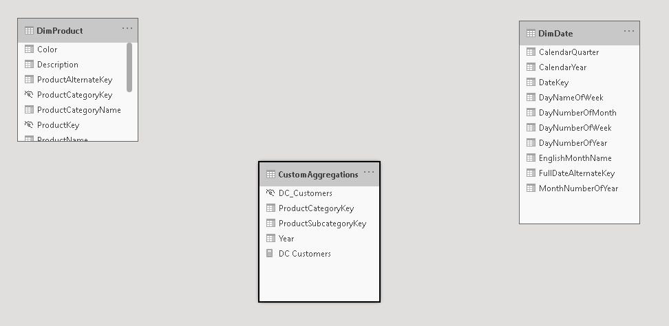
Then relationships are set up between these tables:
In your report you can now simply use the column from the field parameters and add a slicer for the Language table to control which language is displayed. Note: this must be a single-select slicer as otherwise Power BI will build a hierarchy of the different languages!
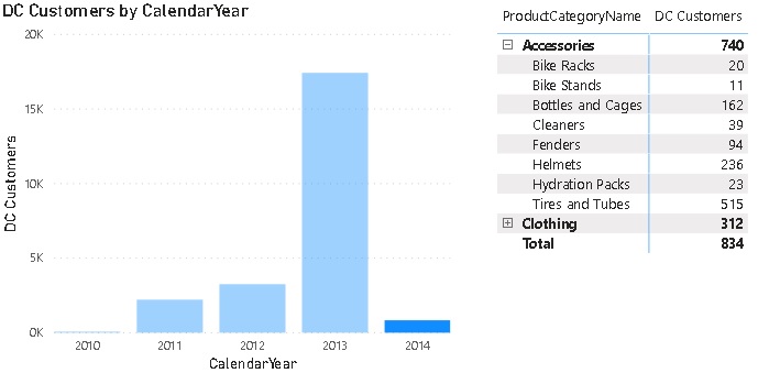
Here is the final result:
(please use Full Screen mode from bottom right corner)
As you can see, we just created a single report that supports multiple languages for both, metadata and data values, allows you to easily switch between them and provides similar performance as if you would have built the report for a single language only!
There are still some open questions when it comes to translating all the labels used on the whole report which is already partially covered in the other blog posts referenced above but this approach brings us another step further to a fully translatable report.
Another nice feature of this approach is that you can also put security on top of the Language/Culture table so a user only sees exactly one row – the one with the language/culture of his choice or country. So a user would not even need to select the language but it would be selected for him automatically!Ideally you could even use the USERCULTURE() DAX function but unfortunately this is currently not supported in the PBI service. There is already an open idea for which you can vote if this is important to you.
USERCULTUER() DAX function is now finally general available also in the service: https://powerbi.microsoft.com/en-us/blog/userculture-dax-function-now-supported-in-power-bi-premium/
The .pbix file can be downloaded here: PBI_Translations.pbix