Upcoming Events I am speaking at in June 2015

I am very glad that I got selected as a speaker for two upcoming SQL Saturdays in June. First there is the SQL Saturday #409 in Rheinland, Germany  on June 13 and the week after the SQL Saturday #419 in Bratislava, Slovakia on June 20.

For those of you who are new to the concept of PASS SQL Saturdays, this is a series of free-of-charge events all around the globe where experienced speakers talk about all topics around the Microsoft SQL Server platform and beyond. As I said, its free, you just need to register in time in order to get a ticked so better be fast before all slots are taken!

SQLSaturday_409_Rheinland_Germany

I will do a session together with my colleague Markus Begerow (b, t) on “Power BI on SAP HANA” – two technologies I got to work a lot with recently. We are going to share our experience on how to use Power BI to extract data from SAP HANA, the different interfaces you can use and the advantages and drawbacks of each. Even tough it is considered a general sessions, we will also do a lot of hands on and elaborate on some of the technical details you need to be aware of, for both, the Power BI side and also for SAP HANA.


SQLSaturday_419_Bratislava_Slovakia

In Bratislava I will speak about Lessons Learned: SSAS Tabular in the real world where I will present the technical and non-technical findings I made in the past when implementing SSAS Tabular models at larger scales for various customers. I will cover the whole process from choosing SSAS Tabular as your engine (or not choosing it), things to consider during implementation and also shed some light on the administrative challenges once the solution is in production.

I think both are really interesting sessions and I would be happy to see a lot of you there and have some interesting discussions!

Recursive Calculations in PowerPivot using DAX

If you have ever tried to implement a recursive calculations in DAX similar to how you would have done it back in the good old days of MDX (see here) you would probably have come up with a DAX formula similar to the one below:

  1. Sales ForeCast :=
  2. IF (
  3.     NOT ( ISBLANK ( [Sales] ) ),
  4.     [Sales],
  5.     CALCULATE (
  6.         [Sales ForeCast],
  7.         DATEADD ( 'Date'[Calendar], 1, MONTH )
  8.     ) * 1.05
  9. )

However, in DAX you would end up with the following error:

A circular dependency was detected: ‘Sales'[Sales ForeCast],’Sales'[Sales ForeCast].

This makes sense as you cannot reference a variable within its own definition – e.g. X = X + 1 cannot be defined from a mathematical point of view (at least according to my limited math skills). MDX is somehow special here where the SSAS engine takes care of this recursion by taking the IF() into account.

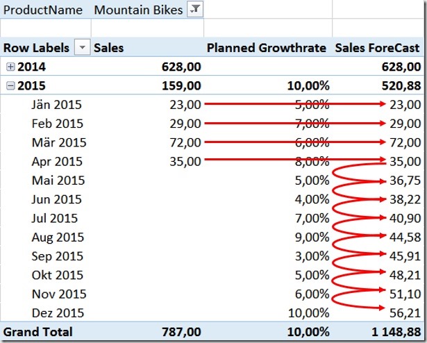
So where could you possible need a recursive calculation like this? In my example I will do some very basic forecasting based on monthly growth rates. I have a table with my actual sales and another table for my expected monthly growth as percentages. If I do not have any actual sales I want to use my expected monthly growth to calculate my forecast starting with my last actual sales:

GeneralLogic

This is a very common requirement for finance applications, its is very easy to achieve in pure Excel but very though to do in DAX as you probably realized on your own what finally led you here Smile

In Excel we would simply add a calculation like this and propagate it down to all rows:
ExcelFormula
(assuming column C contains your Sales, D your Planned Growth Rate and M is the column where the formula itself resides)

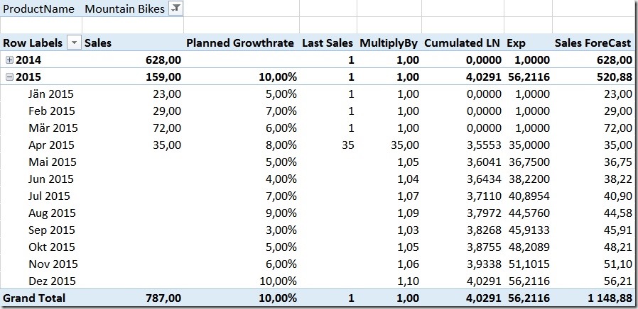
In order to solve this in DAX we have to completely rewrite our calculation! The general approach that we are going to use was already explained by Mosha Pasumansky some years back, but for MDX. So I adopted the logic and changed it accordingly to also work with DAX. I split down the solution into several steps:
1) find the last actual sales – April 2015 with a value of 35
2) find out with which value we have to multiply our previous months value to get the current month’s Forecast
3) calculate the natural logarithm (DAX LN()-function) of the value in step 2)
4) Sum all values from the beginning of time until the current month
5) Raise our sum-value from step 4) to the power of [e] using DAX EXP()-function
6) do some cosmetic and display our new value if no actual sales exist and take care of aggregation into higher levels

Note: The new Office 2016 Preview introduces a couple of new DAX functions, including PRODUCTX() which can be used to combine the Steps 3) to 5) into one simple formula without using any complex LN() and EXP() combinations.

Step 1:
We can use this formula to get our last sales:

  1. Last Sales :=
  2. IF (
  3.     ISBLANK (
  4.         CALCULATE (
  5.             [Sales],
  6.             DATEADD ( 'Date'[DateValue], 1, MONTH )
  7.         )
  8.     ),
  9.     [Sales],
  10.     1
  11. )

It basically checks if there are no [Sales] next month. If yes, we use the current [Sales]-value as our [Last Sales], otherwise we use a fixed value of 1 as a multiplication with 1 has no impact on the final result.

Step 2:
Get our multiplier for each month:

  1. MultiplyBy :=
  2. IF (
  3.     ISBLANK ( [Last Sales] ),
  4.     1 + [Planned GrowthRate],
  5.     [Last Sales]
  6. )

If we do not have any [Last Sales], we use our [Planned GrowthRate] to for our later multiplication/summation, otherwise take our [Last Sales]-value.

Step 3 and 4:
As we cannot use “Multiply” as our aggregation we first need to calculate the LN and sum it up from the first month to the current month:

  1. Cumulated LN :=
  2. CALCULATE (
  3.     SUMX ( VALUES ( 'Date'[Month] ), LN ( [MultiplyBy] ) ),
  4.     DATESBETWEEN (
  5.         'Date'[DateValue],
  6.         BLANK (),
  7.         MAX ( 'Date'[DateValue] )
  8.     )
  9. )


Step 5 and 6:
If there are no actual sales, we display our calculated Forecast:

  1. Sales ForeCast :=
  2. SUMX (
  3.     VALUES ( 'Date'[Month] ),
  4.     IF ( ISBLANK ( [Sales] ), EXP ( [Cumulated LN] ), [Sales] )
  5. )

Note that we need to use SUMX over our Months here in order to also get correct subtotals on higher levels, e.g. Years. That’s all the SUMX is necessary for, the IF itself should be self-explaining here.


So here is the final result – check out the last column:
FinalPivot

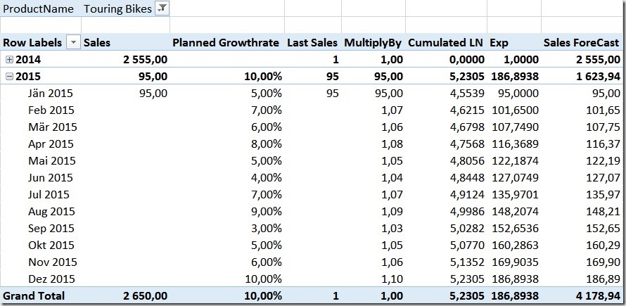
The calculation is flexible enough to handle missing sales. So if for example we would only have sales for January, our recursion would start there and use the [Planned GrowthRate] already to calculate the February Forecast-value:
FinalPivot2

Quite handy, isn’t it?

The sample-workbook (Excel 365) can be downloaded here: RecursiveCalculations.xlsx

Excel CUBE-Functions and MDX UniqueNames

Two weeks ago at the German SQL Server Conference 2015 I was at Peter Myer’s session about Mastering the CUBE Functions in Excel. (PS: Peter is also speaking on our upcoming SQLSaturday #374 in Vienna next week and at PASS SQLRally in Copenhagen the week after). After his session we had a further discussion about this topic and our experiences on how to use Excels CUBE-functions in order to build nice Dashboards with native Excel functionalities that also work with e.g. Excel Services. Its always great to exchange with people that share the same passion on he same topic! One thing we both agreed on that is missing currently is a way to get the MDX UniqueName of something that is selected in a slicer, filter or simply in a cell using CUBEMEMBER-function. I once used a special Cube Measure which was created in MDX Script which returned the UniqueName of a given member that was selected together with this special measure. For this to work with Excel you need to know how Excel builds the MDX when querying cube values using CUBEVALUE-function. Here is a little example:
Excel_CubeValue_Formula
This produces the following MDX query:

  1. SELECT
  2. {
  3.     (
  4.         [Measures].[Internet Sales Amount],
  5.         [Product].[Category].&[1]
  6.     )
  7. } ON 0
  8. FROM [Adventure Works]
  9. CELL PROPERTIES VALUE, FORMAT_STRING, LANGUAGE, BACK_COLOR, FORE_COLOR, FONT_FLAGS

So it basically creates a tuple that contains everything you pass into the CUBEVALUE-Function as a parameter. Knowing this we can create a calculated measure to get the MDX UniqueName of this tuple using MDX StrToTuple()- and MDX AXIS()-function:

  1. MEMBER [Measures].[Excel TupleToStr] AS (
  2. TupleToStr(axis(0).item(0))
  3. )

Replacing the [Measures].[Internet Sales Amount] of our initial CUBEVALUE-function with this new measure would return this to Excel:

  1. ([Measures].[Internet Sales Amount],[Product].[Category].&[1])


Ok, so far so good but nothing really useful as you need to hardcode the member’s UniqueName into the CUBEVALUE-function anyway so you already know the UniqueName.
However, this is not the case if you are dealing with Pivot Table Page Filters and/or Slicers! You can simply refer to them within the CUBEVALUE-function but you never get the UniqueName of the selected item(s). Well, at least not directly! But you can use the approach described above, using an special MDX calculated measure, to achieve this as I will demonstrate on the next pages.

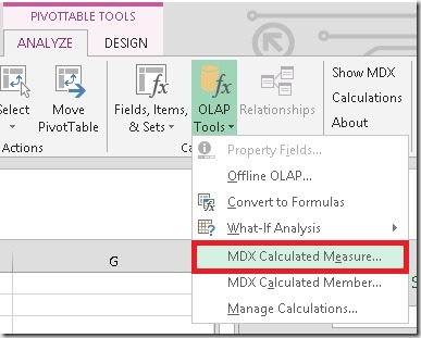
Calculated measures can only be created using the Pivot Table interface but can also be used in CUBE-functions. So first thing you need to do is to create a Pivot Table and add a new MDX Calculated Measure:
Excel_Create_MDX_calculated_measure

!Caution! some weird MDX coming !Caution!


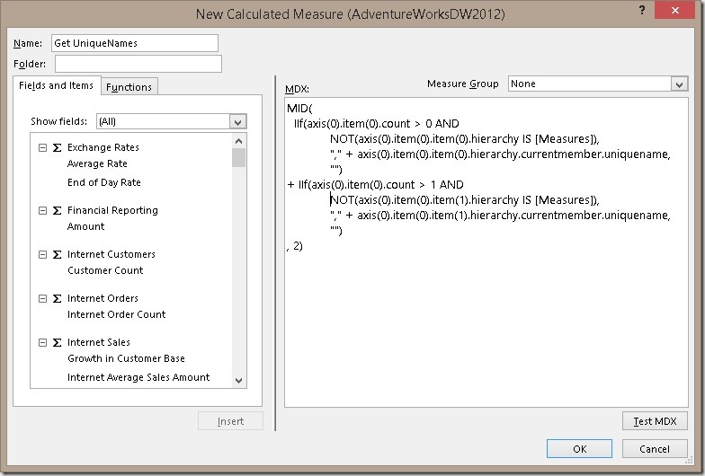
Excel_Create_MDX_calculated_measure2

You may wonder, why such a complex MDX is necessary and what it actually does. What it does is the following: Based on the example MDX query that Excel generates (as shown above) this is a universal MDX that returns the MDX UniqueName of any other member that is selected together with our measure using the CUBEVALUE-function. It also removes the UniqueName of the measure itself so the result can be used again with any other measure, e.g. [Internet Sales Amount]
The reason why it is rather complex is that Excel may group similar queries and execute them as a batch/as one query to avoid too many executions which would slow down the overall performance. So we cannot just reference the first element of our query as it may belong to any other CUBEVALUE-function. This MDX deals with all this kinds of issues.

The MDX above allows you to specify only two additional filters but it may be extended to any number of filters that you pass in to the CUBEMEMBER-function. This would be the general pattern:

  1. MID(
  2.   IIf(axis(0).item(0).count > 0 AND
  3.         NOT(axis(0).item(0).item(0).hierarchy IS [Measures]),
  4.     "," + axis(0).item(0).item(0).hierarchy.currentmember.uniquename,
  5.     "")
  6. + IIf(axis(0).item(0).count > 1 AND
  7.         NOT(axis(0).item(0).item(1).hierarchy IS [Measures]),
  8.     "," + axis(0).item(0).item(1).hierarchy.currentmember.uniquename,
  9.     "")
  10. + IIf(axis(0).item(0).count > n AND
  11.         NOT(axis(0).item(0).item(n).hierarchy IS [Measures]),
  12.     "," + axis(0).item(0).item(n).hierarchy.currentmember.uniquename,
  13.     "")
  14. , 2)

After creating this measure we can now use it in our CUBE-functions in combination with our filters and slicers:
Excel_MDX_CUBEVALUE_UniqueNames_Filter
Excel_MDX_CUBEVALUE_UniqueNames_Slicer

You may noted that I had to use CUBERANKEDMEMBER here. This is because filters and slicers always return a set and if we would pass in a set to our CUBEVALUE function a different MDX query would be generated which would not allow us to extract the single UniqueNames of the selected items using the approach above (or any other MDX I could think of). So, this approach currently only works with single selections! I hope that the Excel team will implement a native function to extract the UniqueName(s) of the selected items in the future to make this workaround obsolete!

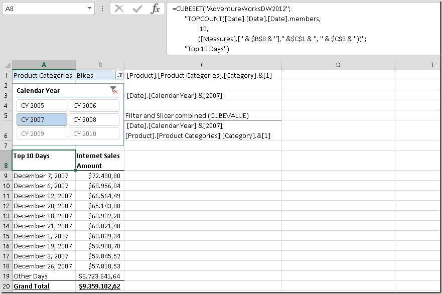
Once we have our UniqeName(s) we can now use them in e.g. a CUBESET-function to return the Top 10 days for a given group of product (filter) and the selected year (slicer):
Excel_MDX_CUBESET_TopCount

And that’s it!

So why is this so cool?

  • It works with SSAS (multidimensional and tabular) and Power Pivot as Excel still uses MDX to query all those sources. It may also work with SAP HANA’s ODBO connector but I have not tested this yet!
  • It does not require any VBA which would not work in Excel Services – this solution does!
  • The calculation is stored within the Excel Workbook so it can be easily shared with other users!
  • There is no native Excel functionality which would allow you to create a simple Top 10 report which works with filters and slicers as shown above or any more complex dynamic report/dashboard with any dynamic filtering.

So no more to say here – Have fun creating your interactive Excel web dashboards!

Download sample Workbook: Samples.xlsx

Note: You may also rewrite any TOPCOUNT expression and use the 4th and 5h parameter of the CUBESET-function instead. This is more native and does not require as much MDX knowledge:Excel_MDX_CUBESET_TopCount_Native
However, if you are not familiar with MDX, I highly recommend to learn it before you write any advanced calculations as show above as otherwise the results might be a bit confusing in the beginning! Especially if you filter and use TOPCOUNT on the same dimension!

Dynamic ABC Analysis in Power Pivot using DAX – Part 2

Almost two years ago I published the first version of an Dynamic ABC Analysis in Power Pivot and by now it is the post with the most comments among all my blog posts. This has two reason:
1) the formula was quite complex and not easy to understand or implement
2) the performance was not really great with bigger datasets

When the first of those comments flew in, I started investigating into a new, advanced formula. At about the same time Marco Russo and Alberto Ferrari published their ABC Classification pattern – a static version using calculated columns – at www.daxpatterns.com. When I had my first dynamic version ready I sent it to Marco and Alberto and asked if they are interested in the pattern and if I can publish it on their website. Long story short – this week the new pattern was released and can now be found here:

ABC Classification – Dynamic

It got some major performance improvements and was also designed towards reusability with other models. The article also contains some detailed explanations how the formula actually works but its still very hard DAX which will take some time to be fully understood. The pattern also features some extended versions to address more specific requirements but I think its best to just read the article on your own.

Hope you enjoy it!

Events-In-Progress for Time Periods in DAX

Calculating the Events-In-Progress is a very common requirement and many of my fellow bloggers like Chris Webb, Alberto Ferrari and Jason Thomas already blogged about it and came up with some really nice solutions. Alberto also wrote a white-paper summing up all their findings which is a must-read for every DAX and Tabular/PowerPivot developer.
However, I recently had a slightly different requirement where I needed to calculate the Events-In-Progress for Time Periods – e.g. the Open Orders in a given month – and not only for a single day. The calculations shown in the white-paper only work for a single day so I had to come up with my own calculation to deal with this particular problem.

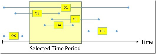
Before we can start we need to identify which orders we actually want to count if a Time Period is selected. Basically we have to differentiate between 6 types of Orders for our calculation and which of them we want to filter or not:
Overview_EventsInProgress_TimeFrame

Order Definition
Order1 (O1) Starts before the Time Period and ends after it
Order2 (O2) Starts before the Time Period and ends in it
Order3 (O3) Starts in the Time Period and ends after it
Order4 (O4) Starts and ends in the Time Period
Order5 (O5) Starts and ends after the Time Period
Order6 (O6) Starts and ends before the Time Period

For my customer an order was considered as “open” if it was open within the selected Time Period, so in our case we need to count only Orders O1, O2, O3 and O4. The first calculation you would usually come up with may look like this:

  1. [MyOpenOrders_FILTER] :=
  2. CALCULATE (
  3.     DISTINCTCOUNT ( ‘Internet Sales’[Sales Order Number] ),
  4.     FILTER (
  5.         ‘Internet Sales’,
  6.         ‘Internet Sales’[Order Date]
  7.             <= CALCULATE ( MAX ( ‘Date’[Date] ) )
  8.     ),
  9.     FILTER (
  10.         ‘Internet Sales’,
  11.         ‘Internet Sales’[Ship Date]
  12.             >= CALCULATE ( MIN ( ‘Date’[Date] ) )
  13.     )
  14. )
[MyOpenOrders_FILTER] :=
CALCULATE (
    DISTINCTCOUNT ( 'Internet Sales'[Sales Order Number] ), -- our calculation, could also be a reference to measure
    FILTER (
        ‘Internet Sales’,
        ‘Internet Sales’[Order Date]
            <= CALCULATE ( MAX ( 'Date'[Date] ) )
    ),
    FILTER (
        ‘Internet Sales’,
        ‘Internet Sales’[Ship Date]
            >= CALCULATE ( MIN ( 'Date'[Date] ) )
    )
)

We apply custom filters here to get all orders that were ordered on or before the last day and were also shipped on or after the first day of the selected Time Period. This is pretty straight forward and works just fine from a business point of view. However, performance could be much better as you probably already guessed if you read Alberto’s white-paper.

So I integrate his logic into my calculation and came up with this formula (Note that I could not use the final Yoda-Solution as I am using a DISTINCTCOUNT here):

  1. [MyOpenOrders_TimePeriod] :=
  2. CALCULATE (
  3.     DISTINCTCOUNT ( ‘Internet Sales’[Sales Order Number] ),
  4.     GENERATE (
  5.         VALUES ( ‘Date’[Date] ),
  6.         FILTER (
  7.             ‘Internet Sales’,
  8.             CONTAINS (
  9.                 DATESBETWEEN (
  10.                     ‘Date’[Date],
  11.                     ‘Internet Sales’[Order Date],
  12.                     ‘Internet Sales’[Ship Date]
  13.                 ),
  14.                 [Date], ‘Date’[Date]
  15.             )
  16.         )
  17.     )
  18. )

To better understand the calculation you may want to rephrase the original requirement to this: “An open order is an order that was open on at least one day in the selected Time Period”.

I am not going to explain the calculations in detail again as the approach was already very well explained by Alberto and the concepts are the very same.

An alternative calculation would also be this one which of course produces the same results but performs “different”:

  1. [MyOpenOrders_TimePeriod2] :=
  2. CALCULATE (
  3.     DISTINCTCOUNT ( ‘Internet Sales’[Sales Order Number] ),
  4.     FILTER (
  5.         GENERATE (
  6.             SUMMARIZE (
  7.                 ‘Internet Sales’,
  8.                 ‘Internet Sales’[Order Date],
  9.                 ‘Internet Sales’[Ship Date]
  10.             ),
  11.             DATESBETWEEN (
  12.                 ‘Date’[Date],
  13.                 ‘Internet Sales’[Order Date],
  14.                 ‘Internet Sales’[Ship Date]
  15.             )
  16.         ),
  17.         CONTAINS ( VALUES ( ‘Date’[Date] ), [Date], ‘Date’[Date] )
  18.     )
  19. )

I said it performs “different” as for all DAX calculations, performance also depends on your model, the data and the distribution and granularity of the data. So you should test which calculation performs best in your scenario. I did a simple comparison in terms of query performance for AdventureWorks and also my customer’s model and results are slightly different:

Calculation (Results in ms)   AdventureWorks   Customer’s Model
[MyOpenOrders_FILTER]                   58.0              1,094.0
[MyOpenOrders_TimePeriod]                   40.0                  390.8
[MyOpenOrders_TimePeriod2]                   35.5                  448.3

As you can see, the original FILTER-calculation performs worst on both models. The last calculation performs better on the small AdventureWorks-Model whereas on my customer’s model (16 Mio rows) the calculation in the middle performs best. So it’s up to you (and your model) which calculation you should prefer.

The neat thing is that all three calculations can be used with any existing hierarchy or column in your Date-table and of course also on the Date-Level as the original calculation.

Download: Events-in-Progress.pbix

Configure HTTP access to Analysis Services using PowerShell

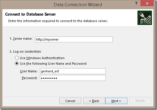
Recently I had to setup an Analysis Services cube and expose it to external users. This is usually done by using Internet Information Server (IIS) and creating a new WebSite which hosts msmdpump.dll. This DLL more or less wraps XMLA commands inside HTTP thus allowing external users to access the cube via HTTP. Besides Windows Authentication this setup also allows Basic Authentication and so external users can simply connect by specifying Username and Password in e.g. Excel when connecting to the cube:
ExcelConnectionDialog

There are already a lot of whitepapers out there which describe how to set things up correctly. Here are just some examples:
– MSDN: http://msdn.microsoft.com/en-us/library/gg492140.aspx
– MSBI Academy (great video!): http://msbiacademy.com/?p=5711 by Rob Kerr

They provide very useful information and you should be familiar with the general setup before proceeding here or using the final PowerShell script.

The PowerShell script basically performs the following steps:

  1. Create a local folder as base for your WebSite in IIS
  2. Copy SSAS ISAPI files (incl. msmdpump.dll) to the folder
  3. Create and Configure an IIS AppPool
  4. Create and Configure a IIS WebSite
  5. Add and enable an ISAPI entry for msmdpump.dll
  6. Configure Authentication
  7. Configure Default Document
  8. Update connection information to SSAS server

I tested it successfully with a clean installation of IIS 8.0 (using applicationhost.config.clean.install). In case you already have other WebSites running you may still consider doing the steps manually or adopting the script if necessary. The script is written not to overwrite any existing Folders, WebSites, etc. but you never know.

So here is my final script:

  1. #Import Modules
  2. Import-Module WebAdministration
  3.  
  4. # change these settings
  5. $iisSiteName = "OLAP"
  6. $iisPort = "8000"
  7. $olapServerName = "server\instance"
  8.  
  9. # optionally also change these settings
  10. $isapiFiles = "c:\Program Files\Microsoft SQL Server\MSAS11.MSSQLSERVER\OLAP\bin\isapi\*"
  11. $iisAbsolutePath = "C:\inetpub\wwwroot\" + $iisSiteName
  12. $iisAppPoolName = $iisSiteName + "_AppPool"
  13. $iisAppPoolUser = "" #default is ApplicationPoolIdentity
  14. $iisAppPoolPassword = ""
  15. $iisAuthAnonymousEnabled = $false
  16. $iisAuthWindowsEnabled = $true
  17. $iisAuthBasicEnabled = $true
  18. $olapSessionTimeout = "3600" #default
  19. $olapConnectionPoolSize = "100" #default
  20.  
  21. if(!(Test-Path $iisAbsolutePath -pathType container))
  22. {
  23.     #Creating Directory
  24.     mkdir $iisAbsolutePath  | Out-Null
  25.  
  26.     #Copying Files
  27.     Write-Host -NoNewline "Copying ISAPI files to IIS Folder … "
  28.     Copy -Path $isapiFiles -Destination $iisAbsolutePath -Recurse
  29.     Write-Host " Done!" -ForegroundColor Green
  30. }
  31. else
  32. {
  33.     Write-Host "Path $iisAbsolutePath already exists! Please delete manually if you want to proceed!" -ForegroundColor Red
  34.     Exit
  35. }
  36.  
  37. #Check if AppPool already exists
  38. if(!(Test-Path $("IIS:\\AppPools\" + $iisAppPoolName) -pathType container))
  39. {
  40.     #Creating AppPool
  41.     Write-Host -NoNewline "Creating ApplicationPool $iisAppPoolName if it does not exist yet … "
  42.     $appPool = New-WebAppPool -Name $iisAppPoolName
  43.     $appPool.managedRuntimeVersion = "v2.0"
  44.     $appPool.managedPipelineMode = "Classic"
  45.  
  46.     $appPool.processModel.identityType = 4 #0=LocalSystem, 1=LocalService, 2=NetworkService, 3=SpecificUser, 4=ApplicationPoolIdentity
  47.     #For details see http://www.iis.net/configreference/system.applicationhost/applicationpools/add/processmodel
  48.  
  49.     if ($iisAppPoolUser -ne "" -AND $iisAppPoolPassword -ne "") {
  50.         Write-Host
  51.         Write-Host "Setting AppPool Identity to $iisAppPoolUser"
  52.         $appPool.processmodel.identityType = 3
  53.         $appPool.processmodel.username = $iisAppPoolUser
  54.         $appPool.processmodel.password = $iisAppPoolPassword
  55.     }
  56.     $appPool | Set-Item
  57.     Write-Host " Done!" -ForegroundColor Green
  58. }
  59. else
  60. {
  61.     Write-Host "AppPool $iisAppPoolName already exists! Please delete manually if you want to proceed!" -ForegroundColor Red
  62.     Exit
  63. }
  64.  
  65. #Check if WebSite already exists
  66. $iisSite = Get-Website $iisSiteName
  67. if ($iisSite -eq $null)
  68. {
  69.     #Creating WebSite
  70.     Write-Host -NoNewline "Creating WebSite $iisSiteName if it does not exist yet … "
  71.     $iisSite = New-WebSite -Name $iisSiteName -PhysicalPath $iisAbsolutePath -ApplicationPool $iisAppPoolName -Port $iisPort
  72.     Write-Host " Done!" -ForegroundColor Green
  73. }
  74. else
  75. {
  76.     Write-Host "WebSite $iisSiteName already exists! Please delete manually if you want to proceed!" -ForegroundColor Red
  77.     Exit
  78. }
  79.  
  80. #Ensuring ISAPI CGI Restriction entry exists for msmdpump.dll
  81. if ((Get-WebConfiguration "/system.webServer/security/isapiCgiRestriction/add[@path='$iisAbsolutePath\msmdpump.dll']") -eq $null)
  82. {
  83.     Write-Host -NoNewline "Adding ISAPI CGI Restriction for $iisAbsolutePath\msmdpump.dll … "
  84.     Add-WebConfiguration "/system.webServer/security/isapiCgiRestriction" -PSPath:IIS:\\  -Value @{path="$iisAbsolutePath\msmdpump.dll"}
  85.     Write-Host " Done!" -ForegroundColor Green
  86. }
  87. #Enabling ISAPI CGI Restriction for msmdpump.dll
  88. Write-Host -NoNewline "Updating existing ISAPI CGI Restriction … "
  89. Set-WebConfiguration "/system.webServer/security/isapiCgiRestriction/add[@path='$iisAbsolutePath\msmdpump.dll']/@allowed" -PSPath:IIS:\\ -Value "True"
  90. Set-WebConfiguration "/system.webServer/security/isapiCgiRestriction/add[@path='$iisAbsolutePath\msmdpump.dll']/@description" -PSPath:IIS:\\ -Value "msmdpump.dll for SSAS"
  91. Write-Host " Done!" -ForegroundColor Green
  92.  
  93.  
  94. #Adding ISAPI Handler to WebSite
  95. Write-Host -NoNewline "Adding ISAPI Handler … "
  96. Add-WebConfiguration /system.webServer/handlers -PSPath $iisSite.PSPath -Value @{name="msmdpump"; path="*.dll"; verb="*"; modules="IsapiModule"; scriptProcessor="$iisAbsolutePath\msmdpump.dll"; resourceType="File"; preCondition="bitness64"}
  97. Write-Host " Done!" -ForegroundColor Green
  98.  
  99. #enable Windows and Basic Authentication
  100. Write-Host -NoNewline "Setting Authentication Providers … "
  101. #need to Unlock sections first
  102. Set-WebConfiguration /system.webServer/security/authentication/anonymousAuthentication  MACHINE/WEBROOT/APPHOST -Metadata overrideMode -Value Allow
  103. Set-WebConfiguration /system.webServer/security/authentication/windowsAuthentication  MACHINE/WEBROOT/APPHOST -Metadata overrideMode -Value Allow
  104. Set-WebConfiguration /system.webServer/security/authentication/basicAuthentication  MACHINE/WEBROOT/APPHOST -Metadata overrideMode -Value Allow
  105.  
  106. Set-WebConfiguration /system.webServer/security/authentication/anonymousAuthentication -PSPath $iisSite.PSPath -Value @{enabled=$iisAuthAnonymousEnabled}
  107. Set-WebConfiguration /system.webServer/security/authentication/windowsAuthentication -PSPath $iisSite.PSPath -Value @{enabled=$iisAuthWindowsEnabled}
  108. Set-WebConfiguration /system.webServer/security/authentication/basicAuthentication -PSPath $iisSite.PSPath -Value @{enabled=$iisAuthBasicEnabled}
  109. Write-Host " Done!" -ForegroundColor Green
  110.  
  111. #Adding Default Document
  112. Write-Host -NoNewline "Adding Default Document msmdpump.dll … "
  113. Add-WebConfiguration /system.webServer/defaultDocument/files -PSPath $iisSite.PSPath -atIndex 0 -Value @{value="msmdpump.dll"}
  114. Write-Host " Done!" -ForegroundColor Green
  115.  
  116. #Updating OLAP Server Settings
  117. Write-Host -NoNewline "Updating OLAP Server Settings … "
  118. [xml]$msmdpump = Get-Content "$iisAbsolutePath\msmdpump.ini"
  119. $msmdpump.ConfigurationSettings.ServerName = $olapServerName
  120. $msmdpump.ConfigurationSettings.SessionTimeout = $olapSessionTimeout
  121. $msmdpump.ConfigurationSettings.ConnectionPoolSize = $olapConnectionPoolSize
  122. $msmdpump.Save("$iisAbsolutePath\msmdpump.ini")
  123. Write-Host " Done!" -ForegroundColor Green
  124.  
  125. Write-Host "Everything done! "
  126. Write-Host "The SSAS server can now be accessed via http://$env:computername`:$iisPort"


The script can also be downloaded here.

The process of setting up HTTP connectivity is the same for Analysis Services Multidimensional and Tabular so the script works for both scenarios, just change the server name accordingly.

Restoring a SSAS Tabular Model to Power Pivot

It is a very common scenario to create a SSAS Tabular Model out of an Power Pivot Model contained in an Excel workbook. Microsoft even created an wizard (or actually a separate Visual Studio project) that supports you doing this. Even further, this process is also a major part of Microsoft’s strategy to cover Personal BI, Team BI and Corporate BI within one technology being xVelocity. This all works just fine but there may also be scenarios where you need to do it the other way round – converting a Tabular model to Power Pivot. Several use-cases come into my mind but I am sure that the most important one is to making data available offline for e.g. sales people to take it with them on their every day work. And in this blog post I will show how this can be done!

But before taking a closer look into how this can be accomplished, lets first see how the import from Power Pivot to SSAS Tabular works. To do this start SQL Server Profiler and connect to your tabular instance. Then create a new Tabular project in Visual Studio based on an existing Power Pivot workbook. At this point you will notice a lot of events happening on our SSAS Tabular server. The most important event for us is “Command End” with the EventSubclass “9 – restore”:
RestoreFromPowerPivot

SSAS actually restores a backup from a “Model.abf” backup file which is located in our project directory that we just created:
BackupExtractedFromPowerPivot

So far so good – but where does this file come from?

Well, the origin of the file has to be our Excel workbook that we imported. Knowing that all new office formats ending with “x” (.xlsx, .docx, …) are basically ZIP files, we can inspect our original Excel workbook by simply rename it to “.zip”. This allows us to browse the Excel file structure:
ExcelUnzipped

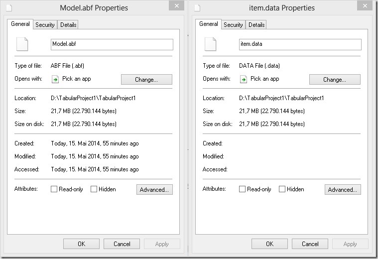
We will find a folder called “xl” which contains a sub-folder called “model”. This folder contains one item called “item.data”. If you take a closer look at the file size you may realize that both, the “Model.abf” file that we restored and the “item.data” file from our Excel workbook have the exact same size:
FileProperties

A Coincidence? Not really!

What happens behind the scenes when you import a Power Pivot model into SSAS Tabular is that this “item.data” file gets copied into your project directory and is renamed to “Model.abf” and then restored to the SSAS Tabular workspace instance by using an standard database restore.

Having this information probably makes you think: If it works in one direction, why wouldn’t it also work the other way round? And it does!

So here are the steps that you need to do in order to restore your SSAS Tabular backup into an Excel Power Pivot workbook:

  1. Create a backup of your SSAS Tabular database and rename it to “item.data”
  2. Create an empty Excel workbook and add a simple linked table to the Excel data model (which is actually Power Pivot).
    This is necessary to tell Excel that the workbook contains a Power Pivot model which has to be loaded once the file is opened.
  3. Close the Excel workbook and rename it from “MyFile.xlsx” to “MyFile.xlsx.zip”
  4. Open the .zip-file in Windows Explorer and locate the “\xl\model\”-folder
  5. Replace the “item.data” file with the file that you created in step 1.
  6. Rename the .zip-file back to “MyFile.xlsx”
  7. Open the Excel Workbook
  8. Voilá! You can now work with the data model as with any other Power Pivot model!

I tested this with a SSAS Tabular backup from SQL Server 2012 SP1 being restored to the streamed version of Excel from Office 365 with the latest version of Power Pivot. I assume that it also works with older versions but have not tested all combinations yet.

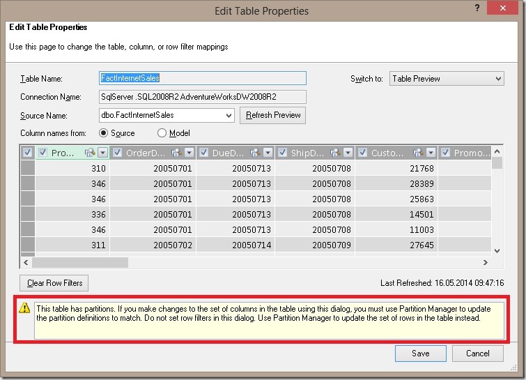
There are also some features that will not work, for example roles. If your Tabular database contains roles you will not be able to use this approach. Excel will complain that the Power Pivot model is broken. However, other Tabular features like partitions actually work with the little limitation that you cannot change them later on in the Power Pivot model or process them separately:
PowerPivotPartitions
Another thing to note here is that only up to 3 partitions are allowed, otherwise you will get the same error as for roles. I think this is related to the limitation of 3 partitions for SQL Server Analysis Services Standard Edition as Chris Webb described here.

Besides these obvious features there are also some other cool things that you can do in Tabular which are not possible in Power Pivot. Most (or actually all) of them are accessible only by using BIDS Helper – a great THANK YOU to the developers of BIDS Helper at this point!
BIDS Helper enables you to add classical multidimensional features also to Tabular models which is not possible using standard Visual Studio only. Those include:

  • DisplayFolders
  • Translations (metadata only)
  • Actions

I tested it for DisplayFolders and Actions and both are working also in Power Pivot after the backup was restored and I further assume that all the other things will also work just fine.
Simply keep in mind that Power Pivot is basically a fully featured Analysis Services instance running within Excel!

For my (and your) convenience I also created a little PowerShell script that does all the work:

  1. # Load the assembly with the ZipFile class
  2. [System.Reflection.Assembly]::LoadWithPartialName("System.IO.Compression.FileSystem") | Out-Null
  3. # Load the assembly to access Analysis Services
  4. [System.Reflection.Assembly]::LoadWithPartialName("Microsoft.AnalysisServices") | Out-Null
  5. # Also install "Analysis Services PowerShell" according to http://technet.microsoft.com/en-us/library/hh213141.aspx
  6.  
  7. # INPUT-Variables, change these to match your environment
  8. $rootFolder = "D:\Test_PowerShell\"
  9. $emptyExcelFile = $rootFolder + "EmptyExcel.xlsx"
  10. $ssasServerName = "localhost\TAB2012"
  11. $ssasDatabaseName = "AdventureWorks"
  12.  
  13. # internal variables
  14. $newExcelFile = $rootFolder + $ssasDatabaseName + ".xlsx"
  15. $newExcelFileZip = $newExcelFile + ".zip"
  16. $unzipFolder = $rootFolder + "TEMP_ExcelUnzipped"
  17. $backupFile = $rootFolder + $ssasDatabaseName + ".abf"
  18. $itemDestination = $unzipFolder + "\xl\model\item.data"
  19.  
  20. # Copy the empty Excel file and rename it to ".zip"
  21. Copy-Item -Path $emptyExcelFile -Destination $newExcelFileZip
  22.  
  23. # Unzip the file using the ZipFile class
  24. [System.IO.Compression.ZipFile]::ExtractToDirectory($newExcelFileZip, $unzipFolder)
  25.  
  26. # Create a backup of the SSAS Tabular database
  27. Backup-ASDatabase -Server $ssasServerName -Name $ssasDatabaseName -BackupFile $backupFile -AllowOverwrite -ApplyCompression
  28.  
  29. # Copy the backup-file to our extracted Excel folder structure
  30. Copy-Item -Path $backupFile -Destination $itemDestination -Force
  31.  
  32. # Check if the target file exists and delete it
  33. if (Test-Path -Path $newExcelFile) { Remove-Item -Path $newExcelFile }
  34.  
  35. # Zip the folder-structure again using the ZipFile class and rename it to ".xlsx"
  36. [System.IO.Compression.ZipFile]::CreateFromDirectory($unzipFolder, $newExcelFile)
  37.  
  38. # Cleanup the unecessary files
  39. Remove-Item -Path $unzipFolder -Recurse
  40. Remove-Item -Path $backupFile
  41. Remove-Item -Path $newExcelFileZip

The last thing to mention here is that I don’t know if this is officially supported in any way by Microsoft – actually I am pretty sure it is not – so watch out what you are doing and don’t complain if something is not working as expected.

Analysis Services Security: Multiple Roles in Tabular vs. Multidimensional – Part 2

In one of my recent posts I highlighted how multiple security roles are handled in tabular opposed to multidimensional Analysis Services models. In this post I will go into more detail and focus on how the security is evaluated for both models.

I would like to continue using the same example as in the last post with the following roles:
“Bikes” – is restricted to [ProductCategory] = “Bikes”
“Brakes” – is restricted to [ProductSubCategory] = “Brakes”
“DE” – is restricted to [Country] = “DE”

I used the following MDX query to test both, the tabular and the multidimensional model:

  1. SELECT
  2. NON EMPTY {[Geography].[Country Region Name].[Country Region Name].MEMBERS} ON 0,
  3. NON EMPTY {[Product].[Product Category Name].[Product Category Name].MEMBERS} ON 1
  4. FROM [Model]
  5. WHERE (
  6. [Measures].[Reseller Total Sales]
  7. )

The last thing I mentioned was how the combination of roles “Bikes” and “DE” could be expressed in SQL:

  1. SELECT
  2.     [ProductCategory],
  3.     [Country],
  4.     SUM([Reseller Sales])
  5. FROM <table>
  6. WHERE [ProductCategory] = ‘Bikes’
  7.     OR [Country] = ‘Germany’
  8. GROUP BY
  9.     [Product Category],
  10.     [Country]


When running the previous MDX query on our tabular model using roles “Bikes” and “DE” we will see a very similar query being executed against our xVelocity Storage Engine:
(Note: There are also some SE engine queries executed to get the elements for rows and columns but the query below is the main query)

  1. SELECT
  2. [Geography_1fa13899-0770-4069-b7cb-5ddf22473324].[EnglishCountryRegionName],
  3. [Product_11920c93-05ae-4f1c-980e-466dfbcfca2a].[CalculatedColumn1 1],
  4. SUM([Reseller Sales_fc635e72-28dc-4156-80d5-43b805f8df1c].[SalesAmount])
  5. FROM [Reseller Sales_fc635e72-28dc-4156-80d5-43b805f8df1c]
  6. LEFT OUTER JOIN [Reseller_d52b9c6f-8d2d-4e23-ae4c-2fc57c1d968a]
  7.         ON [Reseller Sales_fc635e72-28dc-4156-80d5-43b805f8df1c].[ResellerKey]
  8.             =[Reseller_d52b9c6f-8d2d-4e23-ae4c-2fc57c1d968a].[ResellerKey]
  9. LEFT OUTER JOIN [Geography_1fa13899-0770-4069-b7cb-5ddf22473324]
  10.     ON [Reseller_d52b9c6f-8d2d-4e23-ae4c-2fc57c1d968a].[GeographyKey]
  11.         =[Geography_1fa13899-0770-4069-b7cb-5ddf22473324].[GeographyKey]
  12. LEFT OUTER JOIN [Product_11920c93-05ae-4f1c-980e-466dfbcfca2a]
  13.     ON [Reseller Sales_fc635e72-28dc-4156-80d5-43b805f8df1c].[ProductKey]
  14.         =[Product_11920c93-05ae-4f1c-980e-466dfbcfca2a].[ProductKey]
  15. WHERE
  16. (COALESCE((PFDATAID( [Product_11920c93-05ae-4f1c-980e-466dfbcfca2a].[CalculatedColumn1 1] ) = 6))
  17.     OR
  18. COALESCE((PFDATAID( [Geography_1fa13899-0770-4069-b7cb-5ddf22473324].[CountryRegionCode] ) = 5)));

Well, not really readable so lets make it a bit nicer by removing those ugly GUIDs, etc:

  1. SELECT
  2.     [Geography].[EnglishCountryRegionName],
  3.     [Product].[ProductCategory],
  4.     SUM([Reseller Sales].[SalesAmount])
  5. FROM [Reseller Sales]
  6. LEFT OUTER JOIN [Reseller]
  7.     ON [Reseller Sales].[ResellerKey] = [Reseller].[ResellerKey]
  8. LEFT OUTER JOIN [Geography]
  9.     ON [Reseller].[GeographyKey] = [Geography].[GeographyKey]
  10. LEFT OUTER JOIN [Product]
  11.     ON [Reseller Sales].[ProductKey] = [Product].[ProductKey]
  12. WHERE [Product].[ProductCategory] = "Bikes"
  13. OR [Geography].[CountryRegionCode] = "Germany";

This looks very similar to our SQL query. The special thing about it is the WHERE clause which combines the restrictions of both roles using OR which is then propagated also to our [Reseller Sales] fact table and that’s the reason why we see what we want and expect to see – all sales that were either made with “Bikes” OR made in “Germany”:
MultipleRoles_tabular

Another very important thing to note and remember here is that the security restrictions get propagated into and are evaluated within the query. This is done for each and every query (!) which is usually not a problem but may become crucial if you use dynamic security.
To test this with dynamic security I introduced a new role called “CustData” which is going to replace our “Bikes” for this test. It is restricted on table ‘Product’ as:

  1. =([Product Category Name] = IF( CUSTOMDATA() = "1", "Bikes", "Clothing"))

So instead of using the connectionstring “…;Roles=Bikes,DE; …” I now used “…;Roles=CustData,DE;CustomData=1; …” which results in the exact same results of course. However, the query now changed to the following (already beautified) xVelocity query:

  1. SELECT
  2.     [Geography].[EnglishCountryRegionName],
  3.     [Product].[ProductCategory],
  4.     SUM([Reseller Sales].[SalesAmount])
  5. FROM [Reseller Sales]
  6. LEFT OUTER JOIN [Reseller]
  7.     ON [Reseller Sales].[ResellerKey] = [Reseller].[ResellerKey]
  8. LEFT OUTER JOIN [Geography]
  9.     ON [Reseller].[GeographyKey] = [Geography].[GeographyKey]
  10. LEFT OUTER JOIN [Product]
  11.     ON [Reseller Sales].[ProductKey] = [Product].[ProductKey]
  12. WHERE [Product].$ROWFILTER IN '0x000000…000000000000000000000fffff00000000000ffffffff'));
  13. OR [Geography].[CountryRegionCode] = "Germany";

Instead of using a direct filter on [ProductCategory] we now see a filter on $ROWFILTER ?!?

### ASSUMPTIONS START ###
I have to admit that I am currently not entirely sure what this means but I assume the following:
Preceding the main query another xVelocity query is executed which is important for us:

  1. SELECT
  2. [Product].[RowNumber],
  3. [Product].[ProductCategory],
  4. COUNT()
  5. FROM [Product];

This query fetches each [RowNumber] and its associated [ProductCategory]. Internally the [RowNumber] column is created for every table. This is related to the columnar storage that xVelocity uses. Elaborating this in detail would go far beyond the context of this blog post. For more details on the RowNumber-column please refer too http://msdn.microsoft.com/en-us/library/hh622558(v=office.15).aspx which describes the Excel data model which is actually Power Pivot and therefore also applies to Tabular. (In general this link contains a lot of in-depth information on the tabular data model and the columnar storage concepts!)

I further assume that our security-expression is then evaluated against this temporary table to create an bitmap index of which rows match the security-expression and which don’t. This result is then applied to our main query which using the WHERE clause  [Product].$ROWFILTER IN ‘0x0000….’
For all subsequent queries the above query on [RowNumber] and [ProductCategory] is not executed again so I assume that the bitmap index gets cached internally by Analysis Services. I further assume that if the bitmap index gets cached it is also shared between users belonging to the same role which would be similar to multidimensional models.
### ASSUMPTIONS END ###

So the important take-away for tabular is that the security gets propagated into the query and down to the fact table. Combining multiple roles on this level using OR delivers the expected results.


For multidimensional models this is slightly different. You can define security on either the Database Dimension (which gets inherited down to all Cube Dimension) or you can define security on the Cube Dimension directly. Defining security on the Database Dimension already makes it very clear that the security restrictions are independent of any fact table/measure group. A Database Dimension may be used in several cubes so the engine cannot know in advance which measure group to use. Security for multidimensional models is defined on the multidimensional space defined by that dimension. If one role is not restricted on a dimension at all, the user will always see the whole dimension and its associated values, even if a second role would restrict that dimension. And this causes unexpected results as the user may see the whole cube.
In terms of SQL the query could be expressed as:

  1. SELECT
  2.     [ProductCategory],
  3.     [Country],
  4.     SUM([Reseller Sales])
  5. FROM <table>
  6. WHERE ( [ProductCategory] = 'Bikes' OR 1 = 1)
  7.     OR ( 1 = 1  OR [Country] = 'Germany')
  8. GROUP BY
  9.     [Product Category],
  10.     [Country]

The left side of the inner OR statements represents the role “Bikes” whereas the right part represents the “DE” role. It should be very obvious that due to the combination of both roles you finally see everything without any restriction!

Another important thing to point out is that security for multidimensional models is only evaluated once and not for every query. So even if you have complex dynamic security its evaluation only hits you once for the first user that connects to a role and is cached for all queries of that user and also shared with other users belonging to that role.


I hope this gives some more insights on how tabular and multidimensional handle multiple roles and their fundamental differences!

Analysis Services Security: Multiple Roles in Tabular vs. Multidimensional

In terms of security tabular and multidimensional models of SQL Server Analysis Services are very similar. Both use Roles to handle specific security settings. Those Roles are then assigned to users and groups.  This is very trivial if a user only belongs to one Role – the user is allowed to see what is specified in the Role. But it can become very tricky if a user belongs to more than one role.

For both, tabular and multidimensional security settings of multiple roles are additive. This means that you will not see less if you are assigned multiple roles but only more. Lets assume we have the following Roles:
“Bikes” – is restricted to [ProductCategory] = “Bikes”
“Brakes” – is restricted to [ProductSubCategory] = “Brakes”
“DE” – is restricted to [Country] = “DE”

A user belonging to Roles “Bikes” and “Brakes” will see all products that belong to “Bikes” and all products that belong to “Brakes”. This is OK and returns the expected results as  both roles secure the same dimension/table. This applies to tabular and also multidimensional.

However, if roles secure different dimensions/tables it gets a bit more tricky. A user may belong to Roles “Bikes” and “DE”. For multidimensional this is a real problem as it finally result in the user seeing the whole cube! This is “by design” and can be explained as follows:
Role “Bikes” does not have any restriction on [Country] so all countries are visible, Role “DE” has no restriction on [ProductCategory] so all product categories are visible. As Roles are additive the user is allowed to see all countries and also all product categories, hence the whole cube:
MultipleRoles_multidimensional

Basically you would expect to see “Bikes”-sales for all countries and “Germany”-sales for all product categories but you end up seeing much more than this. If you have every faced this problem in real life you know that this is probably not the intended behavior your customers want to see. Usually Active Directory Groups are used and assigned to SSAS roles, so this can happen quite easily without anyone even noticing (except the user who is happy to see more Smile )!
Chris Webb wrote an excellent blog post on how to deal with those kinds of security requirements in multidimensional models here.

For tabular this behavior is somehow similar. A user belonging to both roles is also allowed to see all countries and all product categories – this is because security settings are additive, same as for multidimensional. Even though this is true in terms of the structure (rows, columns) of the query we still get a different result in terms of values!
Here is the same query on a tabular model with the same security settings:
MultipleRoles_tabular

This is exactly what we and our customers would expect to see – all sales for “Germany” and also every sale related to “Bikes”! In tabular models security applied to a given table cascades down to all related tables – in this case to our fact table. If a table is indirectly secured by different Roles which put security on different tables those restrictions are combined using OR. In terms of SQL this could be expressed as:

  1. SELECT
  2.     [ProductCategory],
  3.     [Country],
  4.     SUM([Reseller Sales])
  5. FROM <table>
  6. WHERE [ProductCategory] = 'Bikes'
  7.     OR [Country] = 'Germany'
  8. GROUP BY
  9.     [Product Category],
  10.     [Country]

Further pivoting the result would show the same as the MDX query.

Thinking back to some of my multidimensional cubes where I had to deal with multiple Roles this “slight difference” would have been really handy and would have saved me a lot of time that I put into custom security solutions using bridge tables, assemblies, etc.

In my next post I will go into much more detail on how the tabular security model works so stay tuned!

UPDATE: Part 2 can be found here

Applied Basket Analysis in Power Pivot using DAX

Basket Analysis is a very common analysis especially for online shops. Most online shops make use of it to make you buy products that “Others also bought …”. Whenever you view a specific product “Product A” from the online shop, basket analysis allows the shop to show you further products that other customers bought together with “Product A”. Its basically like taking a look into other customers shopping baskets. In this blog post I will show how this can be done using Power Pivot. Alberto Ferrari already blogged about it here some time ago and showed a solution for Power Pivot v1. There is also dedicated chapter in the whitepaper The Many-to-Many Revolution 2.0 which deals with Basket Analysis, already in Power Pivot v2. Power Pivot v2 already made the formula much more readable and also much faster in terms of performance. Though, there are still some things that I would like to add.

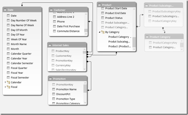
Lets take a look at the initial data model first:Model_Old

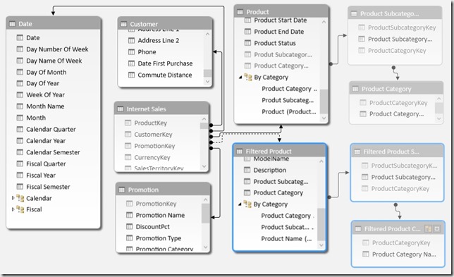
First of all we do not want to modify this model but just extend it so that all previously created measures, calculations and, most important, the reports still work. So the only thing we do is to add our Product-tables again but with a different name. Note that I also added the Subcategory and Category tables in order to allow Basket Analysis also by the Product-Category hierarchy. As we further do not want to break anything we only use an inactive relationship to our ‘Internet Sales’ fact table.

After adding the tables the model looks as follows:Model_New

The next and actually last thing to do is to add the following calculated measure:

Sold in same Order :=
CALCULATE (
COUNTROWS ( ‘Internet Sales’ ),
CALCULATETABLE (
SUMMARIZE (
‘Internet Sales’,
‘Internet Sales’[Sales Order Number]
),
ALL ( ‘Product’ ),
USERELATIONSHIP ( ‘Internet Sales’[ProductKey], ‘Filtered Product’[ProductKey] )
)
)

(formatted using DAX Formatter)

The inner CALCULATETABLE returns a list/table of all [Sales Order Numbers] where a ‘Filtered Product’ was sold and uses this table to extend the filter on the ‘Internet Sales’ table. It is also important to use ALL(‘Product’) here otherwise we would have two filters on the same column ([ProductKey]) which would always result in an empty table. Doing a COUNTROWS finally returns all for all baskets where the filtered product was sold.
We could also change ‘Internet Sales'[Sales Order Number] to ‘Internet Sales'[CustomerKey] in order to analyze what other customers bought also in different baskets (This was done for Example 3). The whole SUMMARIZE-function could also be replaced by VALUES(‘Internet Sales'[Sales Order Number]). I used SUMMARIZE here as I had better experiences with it in terms of performance in the past, though, this may depend on your data. The calculation itself also works with all kind of columns and hierarchies, regardless whether its from table ‘Product’, ‘Filtered Product’, or any other table!

So what can we finally do with this neat formula?

1) Classic Basket Analysis – “Others also bought …”:
Result_ClassicBasketAnalysis

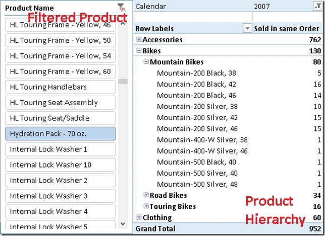
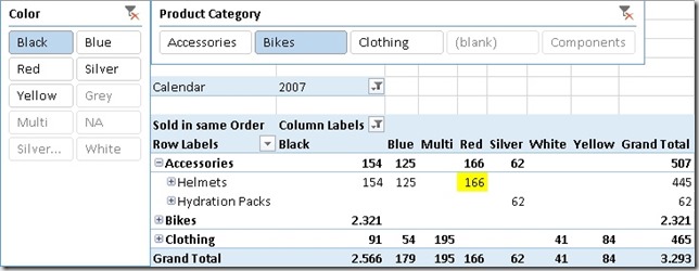
As we can see Hydration Packs are more often sold together with Mountain Bikes opposed to Road Bikes and Touring Bikes. We could also use a slicer on ‘Filtered Product Subcategory’=”Accessories” in order to see how often Accessories are sold together with other products. You may analyze by Color and Product Category:
Result_ByColor
As we can see people that buy black bikes are more likely to buy red helmets than blue helmets.

2) Basket Analysis Matrix:
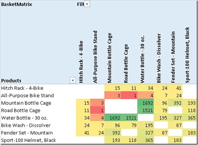
What may also be important for us is which products are sold together the most often? This can be achieved by pulling ‘Product’ on rows and ‘Filtered Product’ on columns. By further applying conditional formatting we can identify correlations pretty easy:
Result_BasketMatrix
Water Bottles are very often sold together with Bottle Cages – well, not really a surprise. Again, you can also use all kind of hierarchies here for your analysis.
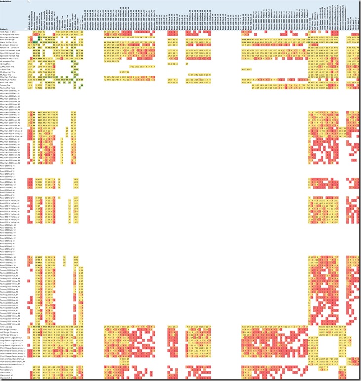
This is what the whole matrix looks like:
Result_BasketMatrixFull
The big blank section in the middle are our Bikes. This tells us that there is no customer that bought two bikes in the same order/basket.

For this analysis I used an extended version of the calculation above to filter out values where ‘Product’ = ‘Filtered Product’ as of course every product is sold within its own basket:

BasketMatrix :=
IF (
MIN ( ‘Product’[ProductKey] )
<> MIN ( ‘Filtered Product’[ProductKey] ),
[Sold in same Order]
)

3) Find Customers that have not bough a common product yet
As we now know from the above analysis which products are very often bought together we can also analyze which customers do not fall in this pattern – e.g. customers who have bough a Water Bottle but have not bought a Bottle Cage yet. Again we can extend our base-calculation to achieve this:

Not Sold to same Customer :=
IF (
NOT ( ISBLANK ( [Sum SA] ) ) && NOT ( [Sold to same Customer] ),
“Not Sold Yet”
)

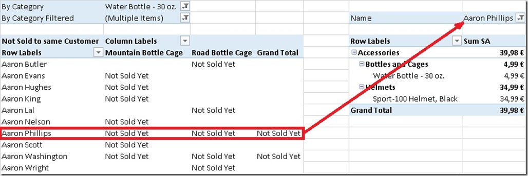
The first part checks if the selected ‘Product’ was sold to the customer at all and the second part checks if the ‘Filtered Product’ was not sold to the customer yet. In that case we return “Not Sold Yet”, and otherwise  BLANK() which is the default if the third parameter is omitted. That’s the result:
Result_NotSoldToCustomer
Aaron Phillips has bought a Water Bottle but no Mountain Bottle Cage nor a Road Bottle Cage – maybe we should send him some advertisement material on Bottle Cages? Smile


As you can see there are a lot of analyses possible on top of that little measure that we created originally. All work with any kind of grouping or hierarchy that you may have and no change to your data model is necessary, just a little extension.

And that’s it – Basket Analysis made easy using Power Pivot and DAX!

Downloads:

Sample Excel Workbook with all Examples: BasketAnalysis.xlsx
Sample PowerBI Desktop file with all Examples (DAX only, no Visuals): BasketAnalysis.pbix