Visualizing SSAS Calculation Dependencies using PowerBI


UPDATE: This does not work for Tabular Models in Compatibility Level 120 or above as they do not expose the calculation dependencies anymore!


One of my best practices when designing bigger SQL Server Analysis Services (SSAS) Tabular models is to nest calculations whenever possible. The reasons for this should be quite obvious:

  • no duplication of logics
  • easier to develop and maintain
  • (caching)

However, this also comes with a slight drawback: after having created multiple layers of nested calculations it can be quite hart to tell on which measures a top-level calculations actually depends on. Fortunately the SSAS engine exposes this calculation dependencies in one of its DMVs – DISCOVER_CALC_DEPENDENCY.
This DMV basically contains information about all calculations in the model:

  • Calculated Measures
  • Calculated Columns
  • Relationships
  • Dependencies to Tables/Columns

Chris Webb already blogged about this DMV some time ago and showed some basic (tabular) visualization within an Excel Pivot table (here). My post focuses on PowerBI and how can make the content of this DMV much more appealing and visualize it in a way that is very easy to understand.
As the DMV is built up like a parent-child hierarchy, I had to use a recursive M-function to resolve this self-referencing table which actually was the hardest part to do. Each row contains a link to a dependent object, which can have other dependencies again. In order to visualize this properly and let the user select a Calculation of his choice to see a calculation tree, I needed to expand each row with all of its dependencies, keeping their link to the root-node:

Here is a little example:

Object Referenced_Object
A B
B C

The table above is resolved to this table:

Root Object Referenced_Object
A A B
A B C
B B C

The Root-column is then used to filter and get all dependent calculations.
The PowerBI file also contains some other M-functions but those are mainly for ease-of-use and to keep the queries simple.

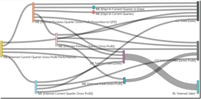
Once all the data was loaded into the model, I could use one of PowerBI’s custom visuals from the PowerBI Gallery – the Sankey Chart with Labels
SSAS_Visualizing_Tabular_Calc_Dependencies

Here is also an interactive version using the Publishing Feature of Power BI:


You can use the Slicers to filter on the Table, the Calculation Type and the Calculation itself and the visual shows all the dependencies down to the physical objects being Tables and Columns. This makes it a lot easier to understand your model and the dependencies that you built up over time.
I attached the sample-PowerBI-file below. You simply need to change the connectionstring to your SSAS Tabular Server and refresh the data connections.

The PowerBI-file (*.pbix) can be downloaded here: SSAS_CalcDependencies.pbix

Using Power BI DMG on Non-Domain Azure VMs – August 2014 Update

In one of my recent posts I explained how to use the Power BI Data Management Gateway to access data hosted in a SQL Server running on an Azure VM. At the time of writing that post the steps to establish connectivity were not quite intuitive. With the latest Update of the Data Management Gateway (Version 1.2.5303.1 and later) things got a bit easier. However, there is still a little thing that you have to configure to make everything work smoothly. First of all, I highly recommend you to read my first post on this topic to fully understand the actual issue and why it does not work out-of-the-box.

When creating a new Data Source the DMG has to be reachable from the machine on which the Data Source Manager (the Click-Once application where you enter your SQL credentials) is executed. The hostname is derived from the DMG and for Azure VMs this does by default not reflect the hostname under which the VM is reachable from public. The hostname would be “MyServer” whereas the public DNS name is “MyServer.cloudapp.net”. To check what hostname the DMG is using you can execute the following Power Shell command:

  1. [System.Net.Dns]::GetHostEntry("localhost")

In order to change this hostname you can either join the VM to a domain (which is not what we want to do here) or use the following approach:

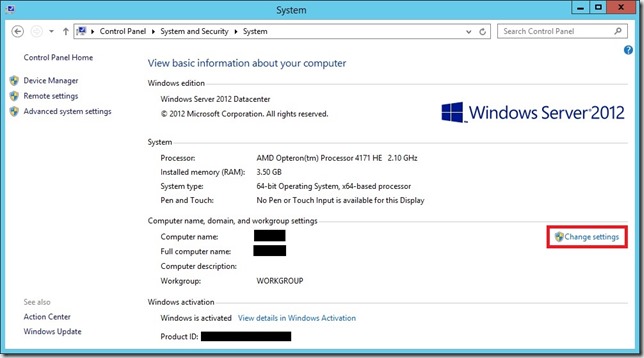
Open the System settings of your server:
SystemSettings_default
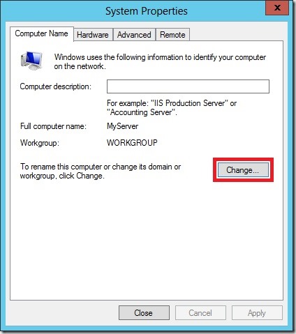
You will notice that both, “Computer name” and “Full computer name” show the same name, and both without the suffix “.cloudapp.net”. In order to change this we need to click the “Change settings” button right next to the names to open the System Properties:
SystemProperties

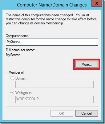
Again, click [Change …] to open the computers domain settings:
DomainSettings
As you can see, the “Full computer name” does not show our required suffix “.cloudapp.net” yet. We can change this in the dialog available via the [More …] Button:
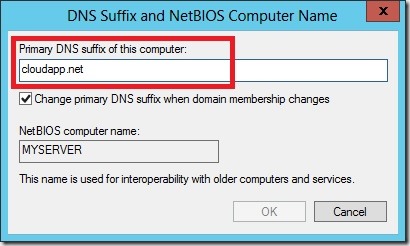
DNS_Settings
Here we can set our “Primary DNS suffix” – we set it to “cloudapp.net” (without leading dot) to reflect our public DNS name.

By clicking [OK] on all open windows you will see the new full name “MyServer.cloudapp.net” now being used as “Full computer name” everywhere. Also our Power Shell command from above now shows the correct hostname. Note that this change also requires a reboot of the VM.

Once the machine is rebooted and DMG is running again you can now use any client machine to create your Data Source which was previously only possible from the server directly and required a RDP connection. Also HTTPS connectivity with self-signed certificates works with this approach which I will show in one of my next posts – so stay tuned!

Using Power BI Data Management Gateway on Non-Domain Azure VM

UPDATE AUGUST 2014:
There were some changes to the DMG in August 2014. Please refer to my new blog post which addresses the issues with the new version! However, I still recommend you to read this post first in order to fully understand the original issue!
The new post can be found here.


I am currently preparing some demos and examples for Power BI. As you can expect for demos you do not want to put too much effort in building up any infrastructure so I decided to use an Azure VM to host my SQL databases and SSAS cubes. Keeping things simple the Azure VM is not joined to a domain which is fine for SQL where I can use SQL authentication, for SSAS I use msmdpump.dll. After everything was set up I wanted to install the Data Management Gateway to expose my SQL tables via OData to Power Query and Online Search.
Bryan C. Smith recently published an article on that very same topic Creating a Demo Power BI Data Gateway using an Azure Virtual Machine but for some reasons it did not work for me. Further, as Bryan already mentions in the first paragraph, his setup is not supported and  its also a bit of a hack (modifying hosts-file, and so on).
So I started my own investigations and came up with another solution, which only uses out-of-the-box features and tools and is actually quite simple. Another thing to mention here is that it will (probably) not work for scheduled data refreshes but only for exposing the SQL database via OData and make it searchable in Power Query.
Having that said, here are the steps to follow:

1) Setup the Data Management Gateway itself on the Azure VM as described here: Create a Data Management Gateway. This should work just fine and the Gateway should be in the “Registered”-state on the Azure VM and in “Ready”-state in the Power BI Admin Center:
 AdminCenter_GW_Ready

2) Create a new Data Source on top of the previously created Gateway as described here: Create a Data Source and Enable OData Feed in Power BI Admin Center

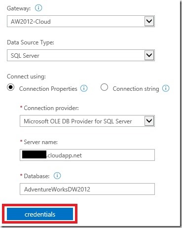
Here you will usually receive an error when you want to enter credentials for the SQL Database:
AdminCenter_DS

By Clicking on the [credentials]-button a new window pops up. Please note that this is a click-once application that actually runs on your client and is independent of your actual browser!
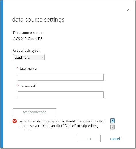
DataSource_Error

If the Gateway is running on an Azure VM, or basically any machine which cannot be reached from your current client you will receive an error that a connection could not be established or something similar.
Assuming you called your Azure VM “MyCloudServer” and is perfectly reachable via “MyCloudServer.cloudapp.net” you will receive an error saying that “MyCloudServer” (without “.cloudapp.net”) could not be resolved. Which is actually true as the correct server would be “MyCloudServer.cloudapp.net”. Unfortunatelly, this server name cannot be changed anywhere as far as I know. As the name cannot be changed we need to make the name somehow “resolveable”. Bryan manually modifies the hosts file and makes “MyCloudServer” point to the public IP address of “MyCloudServer.cloudapp.net”. This should usually work just fine, but somehow did not work for me. Also the public IP address may change if you reboot your Azure VM and so you would need to modify the hosts-file again.

So these are the findings we mad so far:
– the Data Source Manager is a click-once application which runs on the client
– the client must be able to resolve “MyCloudServer”

After some thinking I ended up with the following:
The only machine in my scenario that can correctly resolve “MyCloudServer” is the Azure VM itself! So instead of running the Data Source Manager on my client I simply connected to the Power BI Admin Center from my server and repeated the steps from above there.
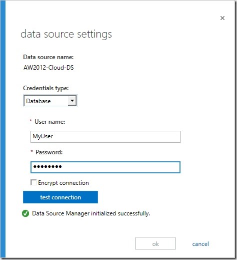
Now everything works fine and we can proceed:
DataSource_Success
This connectivity check is only done once and has no further impact (I am not 100% sure on this Smile ). Though, the Username and Password are stored and used for all subsequent connection through the gateway, e.g. for OData access so make sure the user has the necessary access rights.

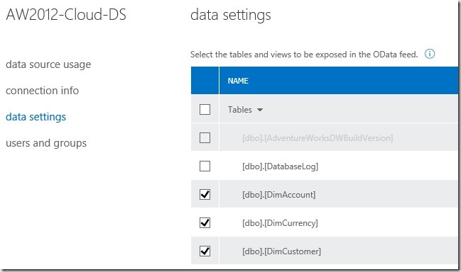
In the next step you can select the tables and views that you want to expose:
DataSource_TablesViews

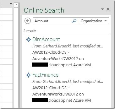
Those can then be searched and queried using Excel and Power Query from any client:
Excel_PowerQuery

And that’s it – The simple trick is to run the Power BI Admin Center from the server itself and create the data source there!

Hope this helps everyone who is dealing with the same issue or wants to setup a demo environment too.

Error-handling in Power Query

Data is the daily bread-and-butter for any analyst. In order to provide good results you also need good data. Sometimes this data is very well prepared beforehand and you can use it as it is but it is also very common that you need to prepare and transform the data on your own. To do this Microsoft has introduced Power Query (on tool of the Power BI suite). Power Query can be used to extract, transform and load data into Excel and/or Power Pivot directly.

When using any data you usually know what the data looks like and what to expect from certain columns – e.g. a value is delivered as a number, a text contains exactly 4 characters, etc.
Though, sometimes this does not apply for all rows of that dataset and your transformation logics may cause errors because of that. In order to avoid this and still have a clean data load you need to handle those errors. Power Query offers several options to this which I will elaborate in this post.

This is the sample data I will use for the following samples:

A B C
1 4 AXI23
2 5 TZ560
NA 6 UP945

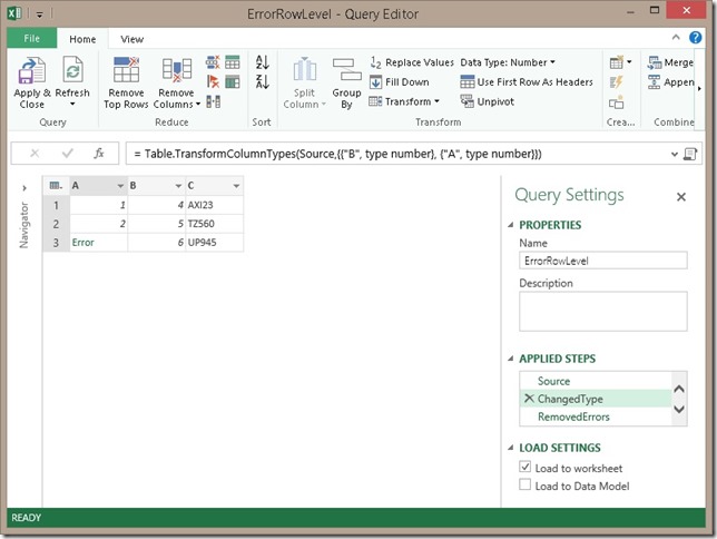
we will perform simple transformations and type casts on this table to generate some errors:

Prepare_ChangeType

Error-handling on row-level

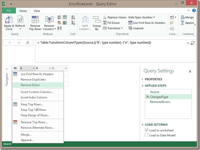
This is the easiest way of handling errors. Whenever a transformation causes an error, we can simply remove the whole row from the result set:

RowLevel_RemoveErrors

This will generate the following result table:

A B C
1 4 AX312
2 5 TZ560

As you can see, the third row was simply removed. This is the easiest way on how to remove errors from your result set but of course this may not be what you want as those removed rows may contain other important information in other columns! Assume you want to calculate the SUM over all values in column B. As we removed the third row we also removed a value from column B and the SUM is not the same as without the error-handling (9 vs. 15)!

Error-handling on cell-level

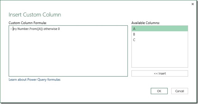
As we now know that column A may result in an error, we can handle this error during our transformation steps. As “NA” could not be converted to a number we see Error as result for that column. Clicking on it gives use some more details on the error itself. To handle this error we need to create a new calculated column where we first check if the value can be converted to a number and otherwise return a default numeric value:

RowLevel_RemoveErrors_CalcColumn

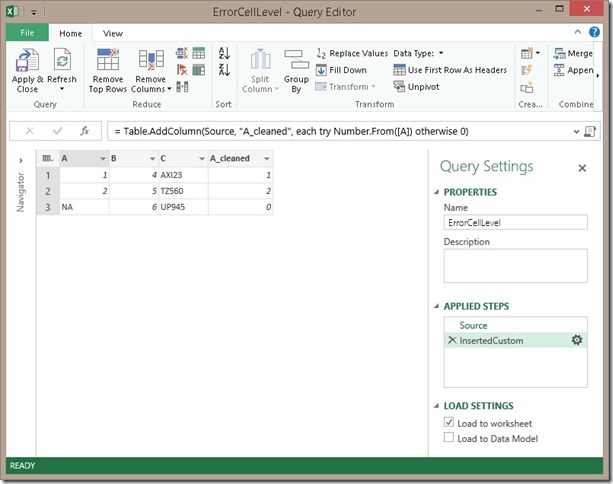
The M-function that we use is “try <expressions to try> otherwise <default if error>” which is very similar to a try-catch block in C#. If the expression causes an error, the default will be used instead. Details on the try-expression can be found in the Microsoft Power Query for Excel Formula Language Specification (PDF) which can be found here and is a must read for everyone interested in the M language.

CellLevel_HandleError

We could further replace our column A by the new column A_cleaned to hide this error handling transformation.

A B C A_cleaned
1 4 AXI23 1
2 5 TZ560 2
NA 6 UP945 0

Error-handling on cell-level with error details

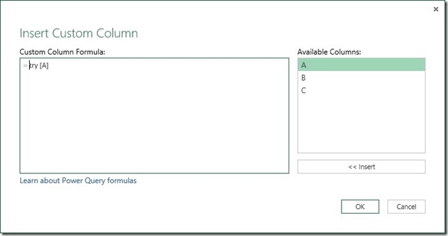
There may also be cases where it is OK to have one of this errors but you need/want to display the cause of the error so that a power user may correct the source data beforehand. Again we can use the try-function, but this time without the otherwise-clause. This will return a record-object for each row:

RowLevel_ShowErrors_CalcColumn

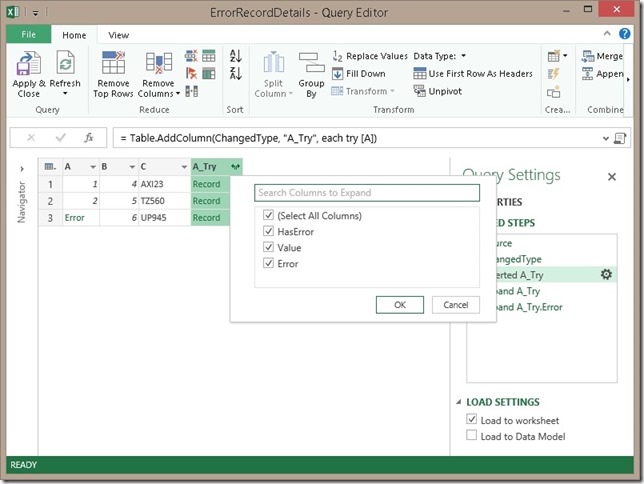
RowLevel_ShowErrors_Result1

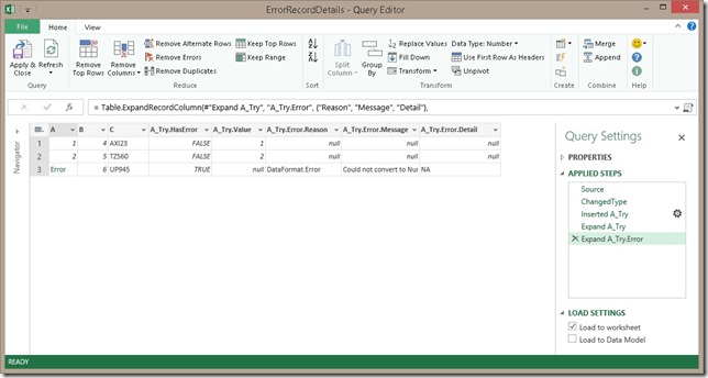
After expanding the A_Try column and also the A_Try.Error column we will get all available information on the error:

RowLevel_ShowErrors_Result2

A B C A_Try.HasError A_Try.Value A_Try.Error.Reason A_Try.Error.Message A_Try.Error.Detail
1 4 AXI23 FALSE 1
2 5 TZ560 FALSE 2
6 UP945 TRUE DataFormat.Error Could not convert to Number. NA

As you can see we get quite a lot of columns here. We could e.g. use A_Try.HasError to filter out error rows (similar to error-handling on row-level) or we could use it in a calculated column to mimic error-handling on cell-level. What you want to do with all the information is up to you, but in case you don’t need it you should remove all unnecessary columns.

Downloads:

Power Query Error Handling Workbook: Power Query Error Handling.xlsx

Using Power Query to analyze SSAS Disk Usage

Some time ago Bob Duffy blogged about on how to use Power Pivot to analyze the disk usage of multidimensional Analysis Services models (here). He uses a an VBA macro to pull meta data like filename, path, extension, etc. from the file system or to be more specific from the data directory of Analysis Services. Analysis Services stores all its data in different files with specific extensions so it is possible to link those files to multidimensional objects in terms of attributes, facts, aggregations, etc. Based on this data we can analyze  how our data is distributed. Do we have too big dimensions? Which attribute uses the most space? Do our facts consume most of the space (very likely)? If yes, how much of it is real data and how big are my aggregations – if they are processed at all?!? – These are very common and also important things to know for an Analysis Services developer.

So Bob Duffy’s solution can be really useful. The only thing I did not like about it was the fact that it uses a VBA macro to get the data. This made me think and I came up with the idea of using Power Query to get this data. Btw, make sure to check out the latest release, there have been a lot of improvements recently!

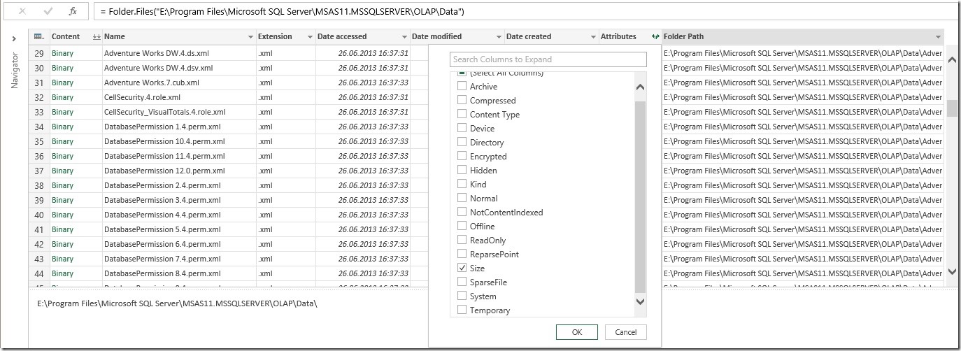
With Power Query you have to option to load multiple files from a folder and also from its sub folders. When we do this on our Analysis Services data directory, we get a list of ALL files together with their full path, filename, extension and most important in this case their size which can be found by expanding the Attributes-record:
PQ_Source_FileList

The final Power Query does also a lot of other things to prepare the data so it can be later joined to our FileExtensions-table that holds detailed information for each file extension. This table currently looks like below but can be extended by any other columns that may be necessary and/or useful for you:

FileType FileType_Description ObjectType ObjectTypeSort ObjectTypeDetails
ahstore Attribute Hash Store Dimensions 20 Attribute
asstore Attribute String Store Dimensions 20 Attribute
astore Attribute Store Dimensions 20 Attribute
bsstore BLOB String Store Dimensions 20 BLOB
bstore BLOB Store Dimensions 20 BLOB
dstore Hierarchy Decoding Store Dimensions 20 Hierarchy
khstore Key Hash Store Dimensions 20 Key
ksstore Key String Store Dimensions 20 Key
kstore Key Store Dimensions 20 Key
lstore Structure Store Dimensions 20 Others
ostore Order Store Dimensions 20 Others
sstore Set Store Dimensions 20 Others
ustore ustore Dimensions 20 Others
xml XML Configuration 999 Configuration
fact.data Basedata Facts 10 Basedata
fact.data.hdr Basedata Header Facts 10 Basedata
fact.map Basedata Index Facts 10 Basedata
fact.map.hdr Basedata Index Header Facts 10 Basedata
rigid.data Rigid Aggregation Data Facts 10 Aggregations
rigid.data.hdr Rigid Aggregation Data Header Facts 10 Aggregations
rigid.map Rigid Aggregation Index Facts 10 Aggregations
rigid.map.hdr Rigid Aggregation Index Header Facts 10 Aggregations
flex.data Flexible Aggregation Data Facts 10 Aggregations
flex.data.hdr Flexible Aggregation Data Header Facts 10 Aggregations
flex.map Flexible Aggregation Index Facts 10 Aggregations
flex.map.hdr Flexible Aggregation Index Header Facts 10 Aggregations
string.data String Data (Distinct Count?) Facts 10 Basedata
cnt.bin Binary Configuration 999 Binaries
mrg.ccmap mrg.ccmap DataMining 999 DataMining
mrg.ccstat mrg.ccstat DataMining 999 DataMining
nb.ccmap nb.ccmap DataMining 999 DataMining
nb.ccstat nb.ccstat DataMining 999 DataMining
dt dt DataMining 999 DataMining
dtavl dtavl DataMining 999 DataMining
dtstr dtstr DataMining 999 DataMining
dmdimhstore dmdimhstore DataMining 999 DataMining
dmdimstore dmdimstore DataMining 999 DataMining
bin Binary Configuration 999 Binaries
OTHERS Others Others 99999 Others

As you can see the extension may contain 1, 2 or 3 parts. The more parts the more specific this file extension is. If you checked the result of the Power Query it also contains 3 columns, FileExtension1, FileExtension2 and FileExtension3. To join the two tables we first need to load both tables into Power Pivot. The next step is to create a proper column on which we can base our relationship. If the 3-part extension is found in the file extensions table, we use it, otherwise we check the 2-part extension and afterwards the 1-part extension and in case nothing matches we use “OTHERS”:

=SWITCH(TRUE(),
CONTAINS(FileTypes, FileTypes[FileType], [FileExtension3]), [FileExtension3],
CONTAINS(FileTypes, FileTypes[FileType], [FileExtension2]), [FileExtension2],
CONTAINS(FileTypes, FileTypes[FileType], [FileExtension1]), [FileExtension1],
"OTHERS")

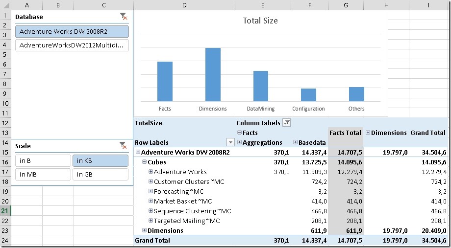
Then we can create a relationship between or PQ table and our file extension table. I also created some other calculated columns, hierarchies and measures for usability. And this is the final outcome:
PivotTable_Report

You can very easily see, how big your facts are, the distribution between base-data and Aggregations, the Dimensions sizes and you can drill down to each individual file! You can of course also create a Power View report if you want to. All visualizations are up to you, this is just a very simple example of a report.

Enjoy playing around with it!

Downloads:
(please note that I added a filter on the Database name as a last step of the Power Query to only show Adventure Works databases! In order to get all databases you need to remove this filter!)

SSAS Disk Analysis Workbook: SSAS_DiskAnalysis.xlsx

SAP HANA’s Big Data Scenario with Power BI

While browsing the web for any BI related topics I recently came across this blog post about SAP HANA and how it can be used to analyze Big Data. Its actually pretty cool, SAP together with Amazon Web Services (AWS) offer a free try out of their tools for 4 hours which you can use to rebuild a predefined demo. The demo itself is very well explained and document with videos and scripts and gives some good insights on how to deal with Big Data in SAP HANA. Basically it is divided into 3 steps:
1) Load Wikipedia data (Pagehits, etc.) from Hadoop/Hive (~2GB of flatfiles)
2) Create a data mart with SAP HANA
3) Analyze results with SAP Lumira

Having done a lot recently with Power BI and its tools I asked myself if this would also be possible with Power BI? So I first did the demo on SAP HANA and afterwards I was quite sure that I could do the same also with Power BI.

And this was the initiation of this blog post where we will do the same demo but instead of SAP HANA we will use only tools of the Power BI suite. Basically we only use 3 of our Power tools:
1) Power Query to load the data
2) Power Pivot to build the “data mart”
3) Power View to analyze the data

First of all we need to load the data. The demo uses data from Wikipedia where for each year, month, day and hour the number of pagehits and bytesdownloaded are monitored per page: http://dumps.wikimedia.org/other/pagecounts-raw/

This data was then moved to a Hadoop/Hive cluster on AWS S3 store which was made public available. The transformed files can be downloaded here (~250MB per file):
http://wikipedia-pagecounts-hive-results.s3.amazonaws.com/year=2013/month=03/000000
http://wikipedia-pagecounts-hive-results.s3.amazonaws.com/year=2013/month=03/000001
http://wikipedia-pagecounts-hive-results.s3.amazonaws.com/year=2013/month=03/000002
http://wikipedia-pagecounts-hive-results.s3.amazonaws.com/year=2013/month=04/000000
http://wikipedia-pagecounts-hive-results.s3.amazonaws.com/year=2013/month=04/000001
http://wikipedia-pagecounts-hive-results.s3.amazonaws.com/year=2013/month=04/000002
http://wikipedia-pagecounts-hive-results.s3.amazonaws.com/year=2013/month=05/000000
http://wikipedia-pagecounts-hive-results.s3.amazonaws.com/year=2013/month=05/000001
http://wikipedia-pagecounts-hive-results.s3.amazonaws.com/year=2013/month=05/000002
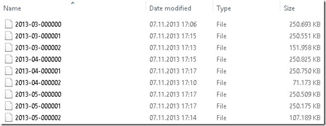
FileList

Once we have downloaded the files we can start loading them using Power Query’s “Load from Folder” source. It is basically textdata which needs to be split into several columns first. The delimiter used is 0x0001 which in Power Query’s M-language needs to be resolved to “#(0001)”:

= Table.SplitColumn(ImportedText ,"Column1",
    Splitter.SplitTextByDelimiter("#(0001)"),
    {"Column1.1", "Column1.2", "Column1.3", "Column1.4",
     "Column1.5", "Column1.6", "Column1.7", "Column1.8"})

The columns are defined as PROJECTCODE, PAGENAME, YEAR, MONTH, DAY, HOUR, PAGEHITCOUNTFORHOUR and BYTESDOWNLOADEDFORHOUR where PROJECTCODE can be further split into language code and the real project code. There is some more logic which I will not explain in detail like error handling, data conversions, etc., which are similar to what is done in the SAP HANA demo.

This is the final M-script I came up with:

let
    Source = Folder.Files("E:\SAP\Big Data"),
    FilteredRows = Table.SelectRows(Source, each ([Extension] = "")),
    CombinedBinaries = Binary.Combine(FilteredRows[Content]),
    ImportedText = Table.FromColumns({Lines.FromBinary(CombinedBinaries)}),
    SplitColumnDelimiter = Table.SplitColumn(ImportedText ,"Column1",Splitter.SplitTextByDelimiter("#(0001)"),{"Column1.1", "Column1.2", "Column1.3", "Column1.4", "Column1.5", "Column1.6", "Column1.7", "Column1.8"}),
    ChangedType = Table.TransformColumnTypes(SplitColumnDelimiter,{{"Column1.1", type text}, {"Column1.2", type text}, {"Column1.3", type number}, {"Column1.4", type number}, {"Column1.5", type number}, {"Column1.6", type number}, {"Column1.7", type number}, {"Column1.8", type number}}),
    SplitColumnDelimiter1 = Table.SplitColumn(ChangedType,"Column1.1",Splitter.SplitTextByDelimiter("."),{"Column1.1.1", "Column1.1.2"}),
    ChangedType1 = Table.TransformColumnTypes(SplitColumnDelimiter1,{{"Column1.1.1", type text}, {"Column1.1.2", type text}}),
    ReplacedValue = Table.ReplaceValue(ChangedType1,null,"wp",Replacer.ReplaceValue,{"Column1.1.2"}),
    InsertedCustom = Table.AddColumn(ReplacedValue, "PageHitsPerHour", each try Number.From([Column1.7]) otherwise 0),
    InsertedCustom1 = Table.AddColumn(InsertedCustom, "BytesDownloadedPerHour", each try Number.From([Column1.8]) otherwise 0),
    RemovedColumns = Table.RemoveColumns(InsertedCustom1,{"Column1.7", "Column1.8"}),
    RenamedColumns = Table.RenameColumns(RemovedColumns,{{"Column1.3", "Year"}, {"Column1.4", "Month"}, {"Column1.5", "Day"}, {"Column1.6", "Hour"}, {"Column1.2", "PageName"}, {"Column1.1.1", "LanguageCode"}, {"Column1.1.2", "ProjectCode"}}),
    InsertedCustom2 = Table.AddColumn(RenamedColumns, "Date", each #date([Year],[Month],[Day])),
    ChangedType2 = Table.TransformColumnTypes(InsertedCustom2,{{"PageHitsPerHour", type number}, {"BytesDownloadedPerHour", type number}, {"Date", type date}}),
    FilteredRows1 = Table.SelectRows(ChangedType2, each [PageHitsPerHour] < 53000000)
in
    FilteredRows1

If you also did the demo on SAP HANA you found some quality issues in the data why you needed to remove rows with more than 53,000,000 PageHitsPerHour as this 5 rows mess up the whole analysis. The above M-script already handles this (last statement).

There are some more important things to mention here. First of all we are dealing with about 37M rows, so loading to datasheet will not work. Instead we need to load the data directly into Power Pivot. I had several memory issues when using 32bit Excel but after switching to a 64bit Excel everything went just fine. The import itself takes about 15 minutes which I think is OK for roughly 2GB of data and 37M rows. 

Once the data is loaded into Power Pivot we need to load some additional data which are basically our lookup/dimension tables. They can also be imported from Wikipedia, in this case directly from the web:
http://wikipedia-proj-lang-codes.s3.amazonaws.com/UniqueProjectCodes.csv
http://wikipedia-proj-lang-codes.s3.amazonaws.com/UniqueLanguageCodes.csv

Both are very simple tables with only two columns. Again we can use Power Query to import them and add them to our Power Pivot data model.

The last thing to add is a time-dimension.SAP HANA has its predefined time-dimension. In the case of Power BI I simply used a linked table in Excel that holds all necessary days or actually all days of 2013. Adding all those tables and linking them we end up with this pretty simple Power Pivot model:
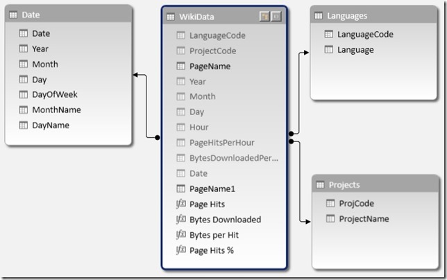
PowerPivot_Diagram

This is very similar to what you create during the demo as an analytical view in SAP HANA so both approaches are very similar here.

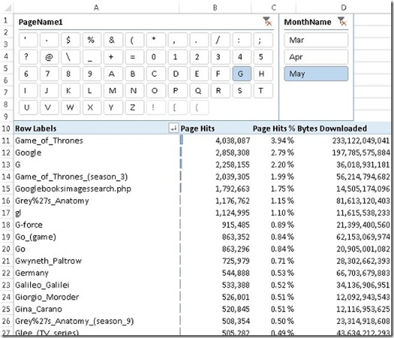
Now that the model is set up we can do our analysis using Power View and classic Excel Pivot Tables:
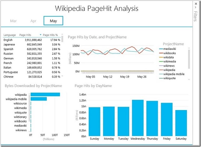
PowerView_Analysis

PivotTable_Report

All together it took me about 2 hours to build the whole solution of which it took about 1h to download and process the data. The final workbook containing all the data has ~500MB which is mainly because of the PageName column which contains a high number of unique values which cannot be compressed very well. After removing the PageName column and some further tuning of the datamodel for compression I could bring the size down to 148 MB. This is quite OK – in numbers this is a compression of 12 from originally 1.74 GB

I hope you understand that I could not attach the whole workbook, instead I created a smaller workbook with only 50k rows by adding a TOP filter in the Power Query. This workbook can be downloaded below.

As I showed in this post, Power BI is capable of handling this kind of data very well. Both, in terms of data volume and also in terms of the type of data (unstructured/semi-structured data). Once the data is loaded into Power Pivot it can be analyzed just like any other data source using all Excel reporting capabilities.

Downloads:
Sample Excel Sheet: Wikidata_small.xlsx
Demo Script SAP HANA: Demo Script SAP HANA.docx
Power Query M-Script: Power Query M-Script.docx